8.3 Asymptotic formulae

8.3.1 Asymptotic form of the MLE

So far, we have discussed how to extract meaningful statistical results from HEP experiments by making extensive use of pseudodata / toy experiments to estimate the sampling distributions of profile-likelihood-ratio-based test statistics. While this worked nicely for our simple counting experiment, generating a sufficiently large number of toys can quickly become computationally intractable for the more complex searches (and statistical combinations of searches) that are increasingly prevalent at the LHC, containing at times up to thousands of bins and nuisance parameters. This and the following section discuss a way to approximate these sampling distributions without the need for pseudodata. This was introduced in the famous “CCGV” paper [301] in 2011 and has since become the de-facto procedure at the LHC.

As hinted at previously, such as in Figures 8.6 and 8.12, the distributions $p({\tilde{t}}_{\mu }|{\mu }^{\prime })$ and $p({\tilde{q}}_{\mu }|{\mu }^{\prime })$ (where, in general, ${\mu }^{\prime }\ne \mu$) have similar forms regardless of the nuisance parameters (or sometimes even the POIs). This is not a coincidence: we will now derive their “asymptotic” — i.e., in the large sample limit — forms, starting first with the asymptotic form of the maximum likelihood estimator (MLE).

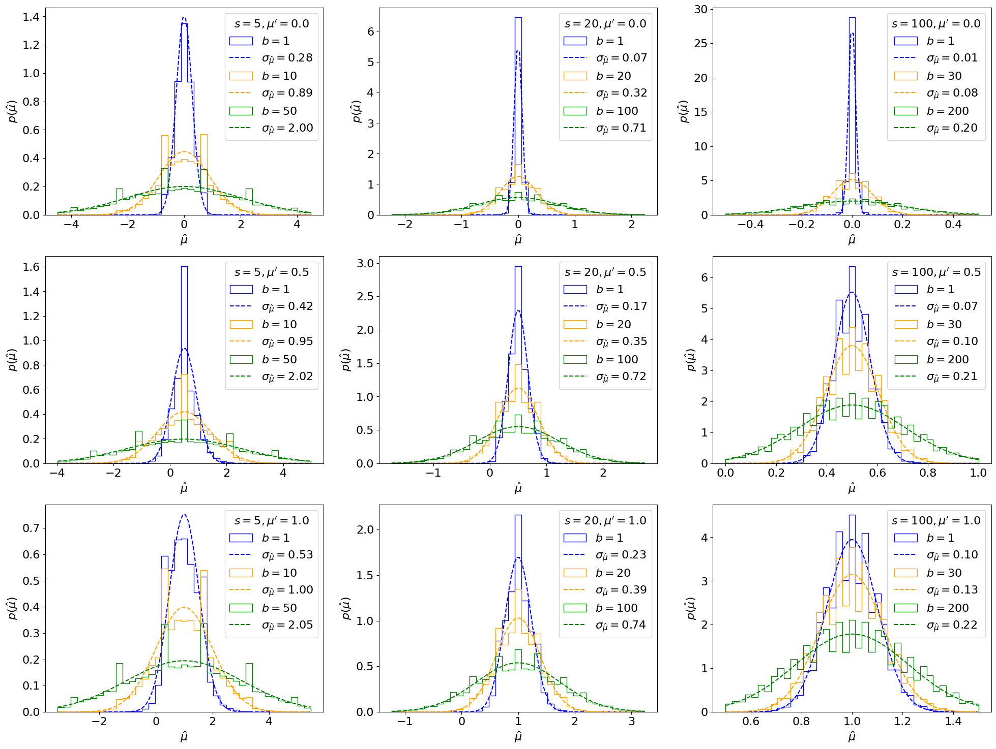
It is important to remember that the MLE $\widehat{\mu }$ of $\mu$ is a random variable with its own probability distribution. We can estimate it as always by sampling toys, shown in Figure 8.20 for our counting experiment (Eq. 8.2.3). One can observe that $p(\widehat{\mu })$ follows a Gaussian distribution as the number of events $N$ increases, and indeed this becomes clear if we try to fit one to the histograms (Figure 8.21). We will now show this to be true generally, deriving the analytic distribution in Sections 8.3.1.—8.3.1., and discussing the results and the important concept of the Asimov dataset for numerical estimation in Sections 8.3.1. and 8.3.1., respectively.

Statistics background

We first provide a lightning review of some necessary statistics concepts and results.

The Fisher information

For our simple counting experiment, the Fisher information matrix $I(\mu ,b)$ can be found by taking second derivatives of the NLL (Eq. 8.2.5). The $I_{\mathit{\mu \mu }}$ term, for example, is:

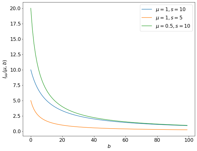
In the last step we use the fact that $𝔼[n]$ under true $\mu ={\mu }^{\prime }$, $b=b^{\prime }$, is ${\mu }^{\prime }s+b^{\prime }$. For the remainder of this section, $I(\mu ,b)$ will always be evaluated at the true values of the parameters,⁶ so this can be simplified to $I_{\mathit{\mu \mu }}({\mu }^{\prime },b^{\prime })=\frac{s^2}{{\mu }^{\prime }s+b^{\prime }}$. This is plotted in Figure 8.22, where we can the Fisher information captures the fact that as $b$ increases, we lose sensitivity to — or information about — $\mu$.

For completeness (and since we’ll need it below), the full Fisher information matrix for our problem, repeating the steps in Eq. 8.3.3, is:

Derivation

We now have enough background to derive the asymptotic form of the MLE. We do this for the 1D case by Taylor-expanding the score of $\widehat{\mu }$, $l^{\prime }(\widehat{\mu })$ - which we know to be $=0$ - around ${\mu }^{\prime }$:

where we plugged in the distribution of $l^{\prime }({\mu }^{\prime })$ from Eq. 8.3.2, claimed $l^{″}({\mu }^{\prime })$ asymptotically equals its expectation value $𝔼[l^{″}({\mu }^{\prime })]=I({\mu }^{\prime })$ by the law of large numbers [307], and are ignoring the $O({(\widehat{\mu }-{\mu }^{\prime })}^2)$ term.⁷

For multiple parameters, $I$ is a matrix so the variance generalized to the matrix inverse:

Result

Thus, we see that $\widehat{\mu }$ asymptotically follows a normal distribution around the true $\mu$ value, ${\mu }^{\prime }$, with a variance ${\sigma }_{\widehat{\mu }}^2=I_{\mathit{\mu \mu }}^{-1}({\mu }^{\prime },b^{\prime })$, up to $O(1∕\sqrt{N})$ terms. Intuitively, from the definition of the Fisher information $I$, we can interpret this as saying that the more information we have about $\mu$ from the data, the lower the variance should be on $\widehat{\mu }$.

Continuing with our counting experiment from Section 8.2.1., inverting $I$ from Eq. 8.3.4 gives us

Note that, as we might expect, this scales as $\sim \sqrt{b}$, which is the uncertainty of our Poisson nuisance parameter $b$ — showing mathematically why we want to keep uncertainties on nuisance parameters as low as possible. This is compared to the toy-based distributions from Section 8.3.1 in Figure 8.23 this time varying the true signal strength ${\mu }^{\prime }$ as well, where we can observe that this matches very well for large $s,b$, while for small values there are some discrete differences.

We can also check the total per-bin errors between the asymptotic form and the toy-based distributions directly, as shown in Figure 8.24 (for ${\mu }^{\prime }=1$ only). Indeed, this confirms that the error scales as $\sim \frac{1}{\sqrt{s}}$ and $\sim \frac{1}{\sqrt{b}}$, as claimed above.

Numerical estimation and the Asimov dataset

In this section, because of the simplicity of our data model, we were able to derive the Fisher information $I$ and, hence, the asymptotic form of $\widehat{\mu }$ analytically. In general, this is not possible and we typically have to minimize $l$, find its second derivatives, and solve Eq. 8.3.3 etc. numerically instead.

However, when calculating the Fisher information, how do we deal with the expectation value over the observed data ($n,m$ in our case)? Naively, this would require averaging over a bunch of generated toy $n,m$ values again, which defeats the purpose of using the asymptotic form of $\widehat{\mu }$!

Instead, we can switch the order of operations in Eq. 8.3.3,⁸ rewriting it as:

Importantly, this says we can find $I$ by simply evaluating the likelihood for a dataset of observations equal to their expectation values under ${\mu }^{\prime }$ instead of averaging over the distribution of observations and then getting its second derivatives.

8.3.2 Asymptotic form of the profile likelihood ratio

We can now proceed to derive the asymptotic form of the sampling distribution $p(t_{\mu }|{\mu }^{\prime })$ of the profile likelihood ratio test statistic $t_{\mu }$, under a “true” signal strength of ${\mu }^{\prime }$. This asymptotic form is extremely useful for simplifying the computation of (expected) significances, limits, and intervals; indeed, standard procedure at the LHC is to use it in lieu of toy-based, empirical distributions for $p(t_{\mu }|{\mu }^{\prime })$.

Asymptotic form of the profile likelihood ratio

We start with deriving the asymptotic form of the profile likelihood ratio test statistic $t_{\mu }$ (Eq. 8.2.7) by following a similar procedure to Section 8.3.1. — and using the results therein — of Taylor expanding around its minimum at $\widehat{\mu }$:¹⁰

Here, just like in Eq. 8.3.6, we use the law of large numbers in Line 8.3.14 and take $l^{″}(\widehat{\mu },\widehat{b})$ to asymptotically equal its expectation value under the true parameter values ${\mu }^{\prime },b^{\prime }$: $l^{″}(\widehat{\mu },\widehat{b})\underset{}{\overset{\sqrt{N}>>1}{\to }}𝔼[l^{″}(\widehat{\mu },\widehat{b})]$. We then in Line 8.3.15 also use the fact that MLEs are generally unbiased estimators of the true parameter values in the large sample limit to say $𝔼[l^{″}(\widehat{\mu },\widehat{b})]\underset{}{\overset{\sqrt{N}>>1}{\to }}𝔼[l^{″}({\mu }^{\prime },b^{\prime })]$. Finally, in the last step, we use the asymptotic form of the MLE (Eq. 8.3.7).

Asymptotic form of $p(t_{\mu }|{\mu }^{\prime })$

Now that we have an expression for $t_{\mu }$, we can consider its sampling distribution. With a simple change of variables, the form of $p(t_{\mu }|{\mu }^{\prime })$ should hopefully be evident: recognizing that $\mu$ and ${\sigma }_{\widehat{\mu }}^2$ are simply constants, while $\widehat{\mu }$ we know is distributed as a Gaussian centered around ${\mu }^{\prime }$ with variance ${\sigma }_{\widehat{\mu }}^2$, let’s define $\gamma \equiv \frac{\mu -\widehat{\mu }}{{\sigma }_{\widehat{\mu }}}$, so that

For the special case of $\mu ={\mu }^{\prime }$, we can see that $t_{\mu }$ is simply the square of a standard normal random variable, which is the definition of the well-known ${\chi }_k^2$ distribution with $k=1$ degrees of freedom (DoF):

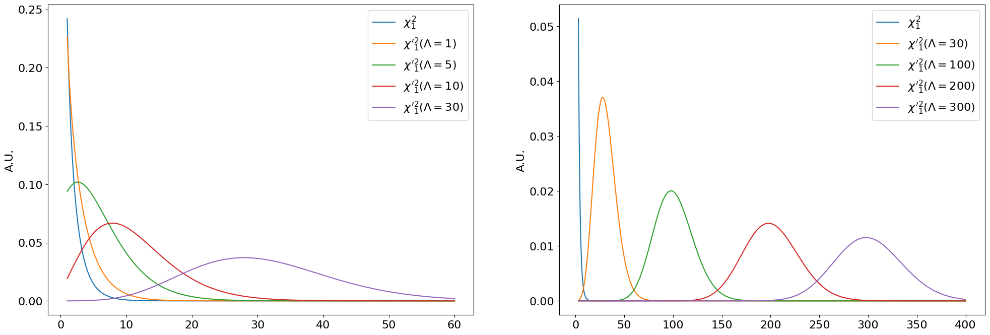
In the general case where $\mu$ may not $={\mu }^{\prime }$, $t_{\mu }$ is the square of random variable with unit variance but non-zero mean. This is distributed as the similar, but perhaps less well-known, non-central chi-squared ${\chi }_k^{\prime 2}(\mathrm{\Lambda })$, again with 1 DoF, and with a “non-centrality parameter”

The “central” vs. non-central chi-squared distributions are visualized in Figure 8.25 for $k=1$. We can see that ${\chi }_k^{\prime 2}(\mathrm{\Lambda })$ simply shifts towards the right as $\mathrm{\Lambda }$ increases (at $\mathrm{\Lambda }=0$ it is a regular central ${\chi }^2$). As $\mathrm{\Lambda }\to \infty$, ${\chi }_k^{\prime 2}(\mathrm{\Lambda })$ becomes more and more like a normal distribution with mean $\mathrm{\Lambda }$.¹¹

By extending the derivation in Eq. 8.3.17 to multiple POIs, one can find the simple generalization to multiple POIs $\mu$:

where the DoF $k$ are equal the number of POIs $\dim <!--\; FUNCTION\; APPLICATION\; -->\mu$, and

where ${\tilde{I}}^{-1}$ is $I^{-1}$ restricted only to the components corresponding to the POIs.

Estimating ${\sigma }_{\widehat{\mu }}^2$

The critical remaining step to understanding the asymptotic distribution of $t_{\mu }$ is estimating ${\sigma }_{\widehat{\mu }}^2$ to find the non-centrality parameter $\mathrm{\Lambda }$ in Eq. 8.3.21. We now discuss two methods to do this.

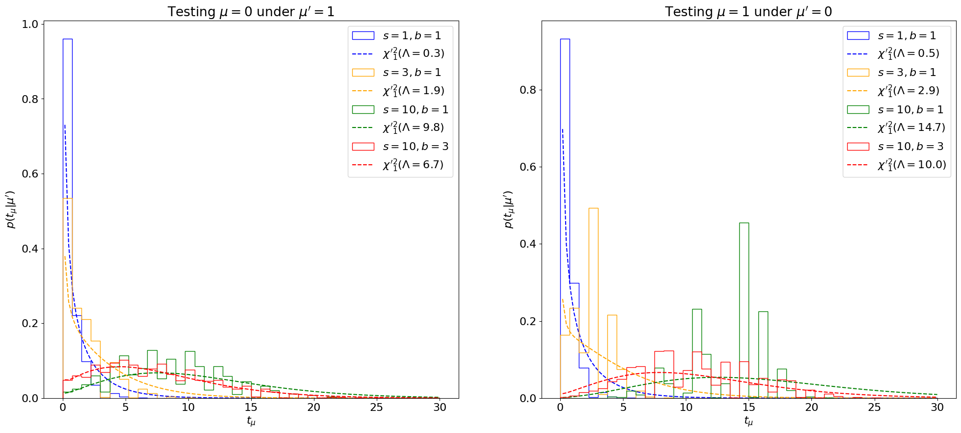
Method 1: Inverting the Fisher information / covariance matrix The first method is simply using ${\sigma }_{\widehat{\mu }}\simeq \sqrt{I_{\mathit{\mu \mu }}^{-1}({\mu }^{\prime },b^{\prime })}$ as in Section 8.3.1.¹² This is shown in Figure 8.26 for our counting experiment, using the analytic form for ${\sigma }_{\widehat{\mu }}$ from Eq. 8.3.8. We can see that this asymptotic approximation agrees well with the true distribution for some range of parameters, but can deviate significantly for others, as highlighted especially in the right plot.

Interlude on Asimov dataset While we are able to find the analytic form for $\sqrt{I_{\mathit{\mu \mu }}^{-1}({\mu }^{\prime },b^{\prime })}$ easily for our simple counting experiment, in general it has to be calculated numerically. As introduced in Section 8.3.1., to handle the expectation value under ${\mu }^{\prime },b^{\prime }$ in Eq. 8.3.1, we can make use of the Asimov dataset, where the observations $n_A$, $m_A$ are taken to be their expectation values under ${\mu }^{\prime },b^{\prime }$, simplifying the calculation of $I$ to Eq. 8.3.9.

Explicitly, for our counting experiment (Eq. 8.2.3), the Asimov observations are simply

We’ll now consider a second powerful use of the Asimov dataset to estimate ${\sigma }_{\widehat{\mu }}^2$.

Method 2: The “Asimov sigma” estimate Putting together Eqs. 8.2.10 and 8.3.26, we can derive a nice property of the Asimov dataset: the MLEs $\widehat{\mu }$, $\widehat{b}$ equal the true values ${\mu }^{\prime }$, $b^{\prime }$:

Thus, $t_{\mu }$ evaluated for the Asimov dataset is exactly the non-centrality parameter $\mathrm{\Lambda }$ that we are after!

While, not strictly necessary to obtain the asymptotic form for $p(t_{\mu }|{\mu }^{\prime })$, we can also invert this to estimate ${\sigma }_{\widehat{\mu }}$, as

where ${\sigma }_A$ is known as the “Asimov sigma”.

The asymptotic distributions using $\mathrm{\Lambda }=t_{\mu ,A}$ are plotted in Figure 8.27. We see that this estimate matches the sampling distributions very well, even for cases where the covariance-matrix-estimate failed! Indeed, this is why estimating ${\sigma }_{\widehat{\mu }}\simeq {\sigma }_A$ is the standard in LHC analyses, and that is the method we’ll employ going forward.

Reference [301] conjectures that this is because the Fisher-information-approach is restricted only to estimating the second-order term of Eq. 8.3.17, while with $t_{\mu ,A}$ we’re matching the shape of the likelihood at the minimum which may be able capture some of the higher order terms as well.

Despite the pervasive use of the asymptotic formula at the LHC, it’s important to remember that it’s an approximation, only valid for large statistics. Figure 8.28 shows it breaking down for $s,b\lesssim 10$ below.

The PDF and CDF

The probability distribution function (PDF) for a ${\chi }_k^{\prime 2}(\mathrm{\Lambda })$ distribution can be found in e.g. Ref. [309] for $k=1$:

where $\phi$ is the PDF of a standard normal distribution. For $\mu ={\mu }^{\prime }\Rightarrow \mathrm{\Lambda }=0$, this simplifies to:

The cumulative distribution function (CDF) for $k=1$ is:

where $\mathrm{\Phi }$ is the CDF of the standard normal distribution. For $\mu ={\mu }^{\prime }\Rightarrow \mathrm{\Lambda }=0$, again this simplifies to:

From Eq. 8.2.14, we know the $p$-value $p_{\mu }$ of the observed $t_{\mu }^{\mathrm{obs}}$ under a signal hypothesis of $H_{\mu }$ is

with an associated significance

Application to hypothesis testing

Let’s see how well this approximation agrees with the toy-based $p$-value we found in Example 8.2.1. For the same counting experiment example, where we expect $s=10$ and observe $n_{\mathrm{obs}}=20$, $m_{\mathrm{obs}}=5$, we found the $p$-value for testing the $\mu =1$ hypothesis $p_{\mu =1}=0.3$ (and the associated significance $Z=0.52$). Calculating $t_{\mu }^{\mathrm{obs}}$ for this example and plugging it into the asymptotic approximation from Eq. 8.3.35 gives:¹³

We see that it agrees exactly!

The agreement more generally, with varying $s,\mu ,n_{\mathrm{obs}},m_{\mathrm{obs}}$, is plotted in Figure 8.29. We observe generally strong agreement, except for low $n,m$ where, as expected, the asymptotic approximation breaks down.

Summary

We have been able to find the asymptotic form for the profile-likelihood-ratio test statistic $t_{\mu }\simeq \frac{{(\mu -\widehat{\mu })}^2}{{\sigma }_{\widehat{\mu }}^2}$, which is distributed as a non-central chi-squared (${\chi }_k^{\prime 2}(\mathrm{\Lambda })$) distribution. We discussed two methods for finding the non-centrality parameter $\mathrm{\Lambda }$, out of which the Asimov sigma ${\sigma }_A$ estimation generally performed better. Finally, the asymptotic formulae were applied to simple examples of hypothesis testing to check the agreement with toy-based significances. These asymptotic formulae can be extended to the alternative test statistics for positive signals ${\tilde{t}}_{\mu }$ and upper-limit-setting ${\tilde{q}}_{\mu }$, as in Ref. [301], to simplify the calculation of both observed and expected significances, limits, and intervals.

With that, we conclude the overview of the statistical interpretation of LHC results. We will see practical applications of these concepts to searches in the high energy Higgs sector in Part V.