

8.2 Frequentist statistics at the LHC
8.2.1 The likelihood function and test statistics
The data model
Let us take the simplest possible case of a (one bin) counting experiment, where in our “signal region” we expect signal events and background events. The probability to observe events in our signal region is distributed as a Poisson with mean :
|
| (8.2.1) |
Since we have only one observation but two free parameters, this experiment is underconstrained. So, let’s also add a “control region” where we expect no signal and background events. The probability of observing events in our control region is therefore:
|
| (8.2.2) |
Combining the two, the joint probability distribution for and is:
|
| (8.2.3) |
This is also called the model for the data and is plotted for sample values in Figure 8.1.
The likelihood function
In the frequentist philosophy, however, all our parameters , etc. are simply fixed values of nature and, hence, don’t have a probability distribution. Instead, we work with the likelihood function, which is a function only of our parameters of interest (POIs), in our example, and “nuisance parameters” (), given fixed values for and :
|
| (8.2.4) |
Importantly, this is not a probability distribution on and ! To derive that, we would have to use Bayes’ rule to go from ; however, such probability distributions don’t make sense in our frequentist world view, so we’re stuck with this likelihood formulation. Often, it’s more convenient to consider the negative log-likelihood:
|
| (8.2.5) |
The profile likelihood ratio
Fundamentally, the goal of any experiment is to test the compatibility of the observed data ( here) with a certain hypothesis . We do this by mapping the data to a “test statistic” , which is just a number, and comparing it against its distribution under , . Our problem, thus, boils down to 1) choosing the most effective for testing , and 2) obtaining .
In the case of testing a particular signal strength, we use the “profile likelihood ratio”:
|
| (8.2.6) |
where are the maximum-likelihood estimates (MLEs) for and , given the observations , and is the MLE for given , and . The MLE for a parameter is simply the value of it for which the likelihood is maximized, and will be discussed in the next section. The numerator of can be thought of as a way to “marginalize” over the nuisance parameters by simply values that maximize the likelihood for any given , while the denominator is effectively a normalization factor, such that .
Again, it’s often more convenient to use the (negative) logarithm:
|
| (8.2.7) |
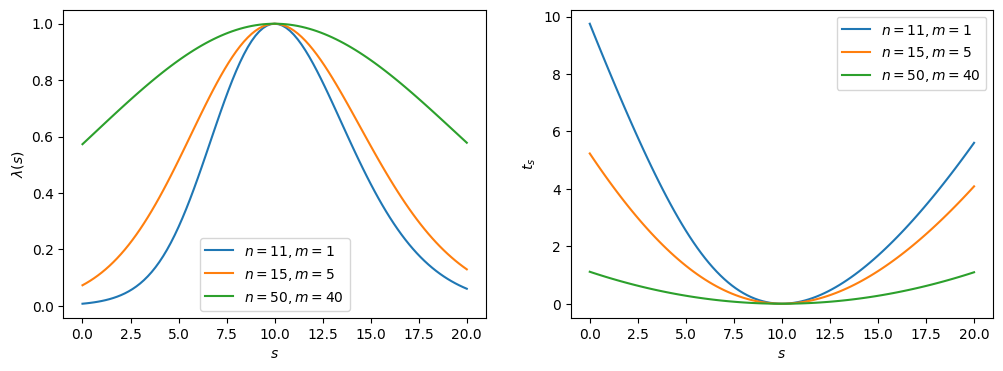
Note that . and are plotted for sample values with in Figure 8.2. The maximum (minimum) of the profile likelihood ratio () is at , as we expect; however, as the ratio between and decreases — i.e., the experiment becomes more noisy — the distributions broaden, representing the reduction in sensitivity, or the higher uncertainty on the true value of .
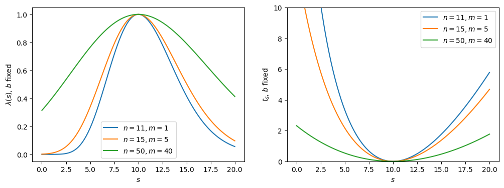
Note that the likelihood ratio and are also broadened due to the nuisance parameter; i.e., because we are missing information about . This can be demonstrated by plotting them with , emulating perfect information of (Figure 8.3), and indeed, we see the functions are narrower than in Figure 8.2. More generally, increasing (decreasing) the uncertainties on the nuisance parameters will broaden (narrow) the test statistic distribution. This is which is why experimentally we want to constrain them through auxiliary measurements as much as possible.
Maximum-likelihood estimates
MLEs for and can be found for this example by setting the derivative of the negative log-likelihood to 0 (more generally, this would require numerical minimization):
Solving simultaneously yields, as you might expect:
|
| (8.2.10) |
Or just for from Eq. 8.2.8:
|
| (8.2.11) |
Plugging this back in, we can get and for any given .
Alternative test statistic
So far, our construction allows for ; however, physically the number of signal events can’t be negative. Rather than incorporating this constraint in the model, it’s more convenient to impose this in the test statistic, by defining:
|
| (8.2.12) |
and
|
| (8.2.13) |
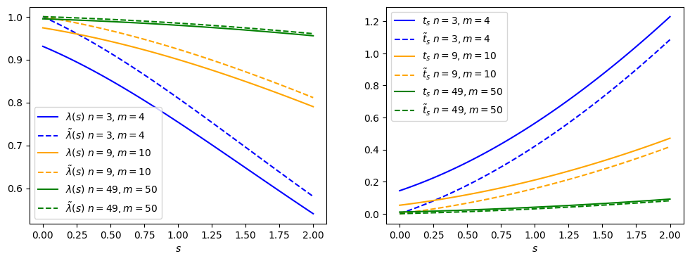
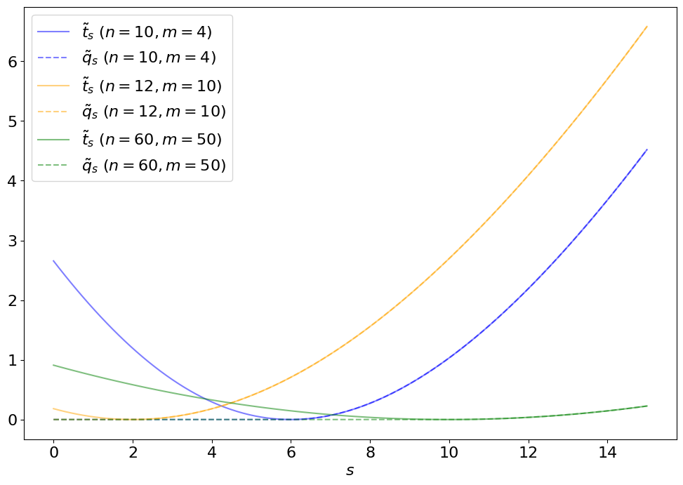
The difference between the nominal and alternative test statistics is highlighted in Figure 8.4. For , the and values are at , since physically that is what fits best with our data (even though the math says otherwise).
Next, we want to translate this to a probability distribution of under a particular signal hypothesis () (i.e., an assumed value of ): , or just for simplicity.
8.2.2 Hypothesis testing
The goal of any experiment is to test whether our data support or exclude a particular hypothesis , and quantify the (dis)agreement. For example, to what degree did our search for the Higgs boson agree or disagree with the standard model hypothesis?
We have already discussed the process of mapping data to a scalar test statistic that we can use to test . However, we need to know the probability distribution of under to quantify the (in)consistency of the observed data with and decide whether or not to exclude .
We must also recognize that there’s always a chance that we will exclude even if it’s true (called a Type I error, or a false positive), or not exclude when it’s false (Type II error, or false negative). The probability of each is referred to as and , respectively. This is summarized handily in Table 8.1.
Before the test, we should decide on a probability of making a Type I error, , that we are comfortable with, called a “significance level”. Typical values are 5% and 1%, although if we’re claiming something crazy like a new particle, we better be very sure this isn’t a false positive; hence, we set a much lower significance level for these tests of . (The significance of this value will be explained in Section 8.2.2. below.)
Deriving
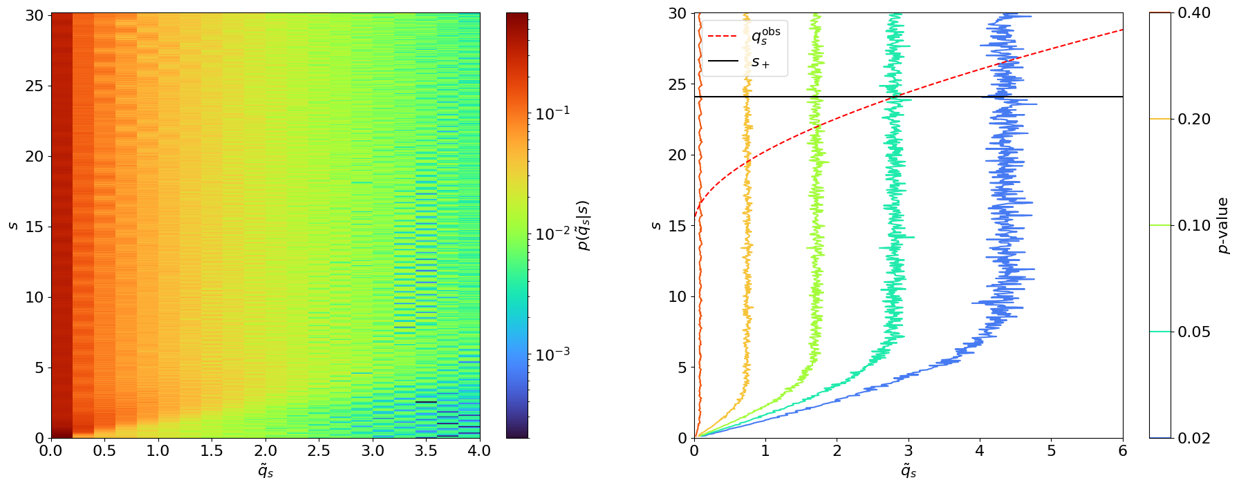
We can approximate by generating several pseudo- or “toy” datasets assuming expected signal events. In this case, this means sampling possible values for from our probability model. We will continue with our simple counting experiment (Section 8.2.1.), for which such toy datasets are generated and then used to create histograms for in Figure 8.5. Note that one complication in generating these toys is that the distributions from which we want to sample (Eq. 8.2.3) also depend on the nuisance parameter . However, we see from the figure that this does not matter as much as we might expect.
We make two important observations:
- 1.
- does not depend on nuisance parameters as long as we have sufficiently large statistics (in this case, when is sufficiently large). This is a key reason for basing our test statistic on the profile likelihood.
- 2.
- In fact, doesn’t even depend on the POI ! (Again, as long as is large.)
Reference [301] shows that, asymptotically, this distribution follows a distribution with degrees of freedom equal to the number of POIs, as illustrated in Figure 8.6.1 We can see that the asymptotic form looks accurate even for as low as . Note that for cases where we can’t use the asymptotic form, Ref. [58] recommends using when generating toys, so that we (approximately) maximize the agreement with the hypothesis.
-values and significance
Now that we know the distribution of the test statistic , we can finally test with our experiment. We just need to calculate the “observed” test statistic from our observations, and compare it to the .
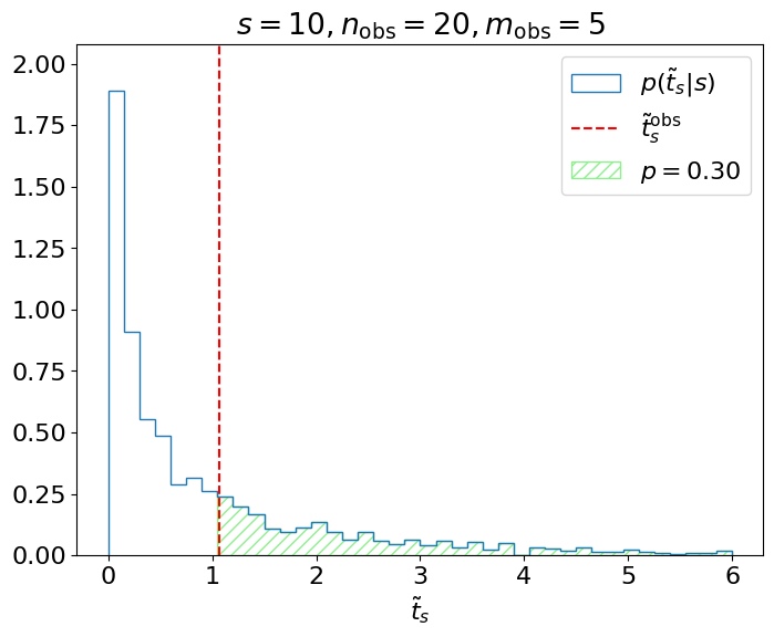
Example 8.2.1. Let’s say we’re testing the hypothesis of signal events in our model and we observe events. We can map this observation to our test statistic , and see where this falls in our distribution (Figure 8.7).
Ultimately, we care about, given , the probability of obtaining or a value more inconsistent with ; i.e., the green shaded region above. This is referred to as the -value of the observation:
|
| (8.2.14) |
which is for this example, where
|
| (8.2.15) |
is the cumulative distribution function (CDF) of . We reject the hypothesis if this -value is less than our chosen significance level ; the idea being that if were true and we repeated this measurement many times, then the probability of a false-positive (-value ) is exactly , as we intended.
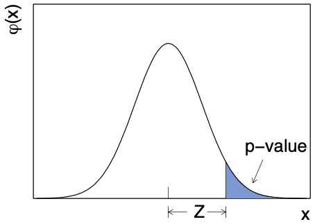
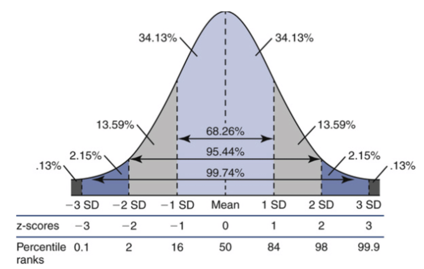
The -value is typically converted into a significance (), which is the corresponding number of standard deviations away from the mean in a Gaussian distribution:
|
| (8.2.16) |
where is the CDF of the standard Gaussian. This is more easily illustrated in Figure 8.8, where is the standard Gaussian distribution:
The significance in Example 8.2.1 is, therefore, . We sometimes say that our measurement is (in)consistent or (in)compatible with at the level, or within , etc.
Signal discovery
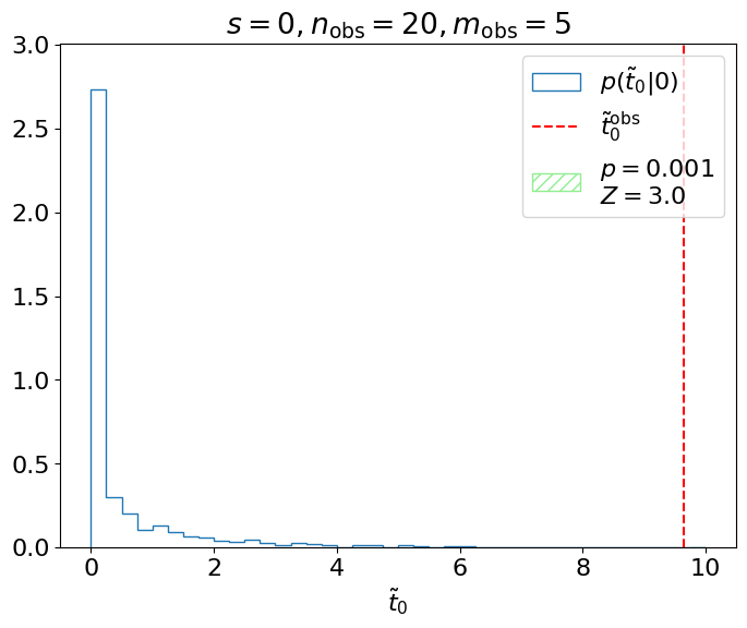
So far, we have been testing the signal hypothesis, but usually when searching for a particle, we instead test the “background-only” hypothesis and decide whether or not to reject it. This means we want and (Figure 8.9).2
We could say for this experiment, therefore, that we exclude the background-only hypothesis at the “3 sigma” level. However, for an actual search for a new particle at the LHC, this is insufficient to claim a discovery, as the probability of a false positive at , 1/1000, is too high. The standard is instead set at for discovering new signals, corresponding to the significance level quoted earlier, as we really don’t want to be making a mistake if we’re claiming to have discovered a new particle! , , and are commonly referred to as “evidence”, “observation”, and “discovery”, respectively, of the signals we’re searching for.
In summary, the framework for hypothesis testing comprises:
- 1.
- Defining a test statistic to map data (in our example, ) to a single number.
- 2.
- Deriving the distribution of under the hypothesis being tested by sampling from “toy” datasets assuming .
- 3.
- Quantifying the compatibility of the observed data with with the -value or significance of relative to .
This -value / significance is what we then use to decide whether or not to exclude . A particularly important special case of this, as discussed above, is testing the background-only hypothesis when trying to discover a signal.
8.2.3 Confidence intervals and limits
Confidence intervals using the Neyman construction
Next, we discuss going beyond hypothesis testing to setting intervals and limits for parameters of interest. The machinery from Section 8.2.2 can be extended straightforwardly to extracting “confidence intervals” for our parameters of interest (POIs): a range of values of the POIs that are allowed, based on the experiment, at a certain “confidence level” (CL), e.g. 68% or 95%. Very similar to the idea of the significance level, the CL is defined such that if we were to repeat the experiment many times, a 95%-confidence-interval must contain, or cover, the true value of the parameter 95% of the time.
This can be ensured for any given CL by solving Eq. 8.2.14 for a -value of :
|
| (8.2.17) |
where and are the lower and upper limits on , respectively.
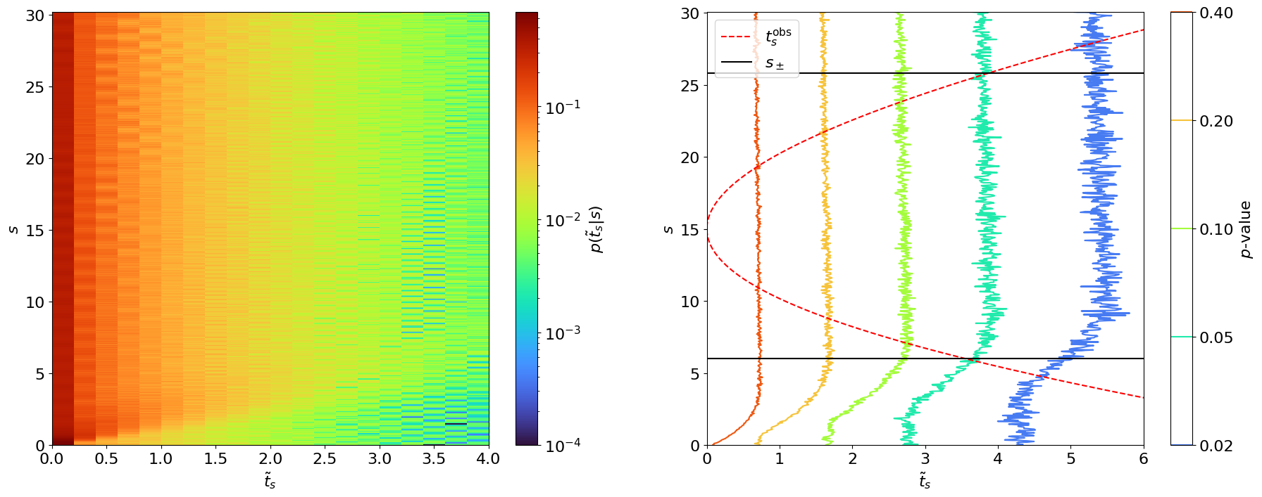
This can be solved by scanning and finding the values of for which the RHS , as demonstrated in Figure 8.10 for the experiment in Example 8.2.1 (). This procedure of inverting the hypothesis test by scanning along the values of the POIs is called the “Neyman construction”.
One subtlety to remember is that, in principle, we should also be scanning over the nuisance parameters () when estimating the -values. However, this would be very computationally expensive so in practice, we continue to use , to always (approximately) maximize the agreement with the hypothesis. Ref. [58] calls this trick “profile construction”.
Upper limits
Typically if a search does not have enough sensitivity to directly observe a new signal, we instead quote an upper limit on the signal strength. This is similar in practice to the Neyman construction for confidence intervals, solving Eq. 8.2.17 only for the upper boundary. However, an important difference is that when setting upper limits, we have to modify the test statistic so that a best-fit signal strength greater than the expected signal () does not lower the compatibility with :
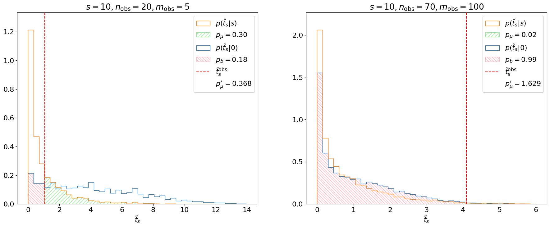
The upper limit test statistic is set to for so that this situation does not contribute to the -value integral in Eq. 8.2.14. Figure 8.11 demonstrates this, and the difference between and , for different sample observations.
Note that (as one may expect from Figure 8.11) the distribution no longer behaves like a standard but, instead, as a “half-”. This is essentially a plus a delta function at 0 (since, under the signal hypothesis, on average there will be an over-fluctuation half the time, for which ), as shown in Figure 8.12.
We can now revisit Example 8.2.1 to set an upper limit on rather than a confidence interval (Figure 8.13). is shifted to the left with respect to ; hence, the upper limit of is slightly lower than the upper bound of the 95% confidence interval we derived using .
The CL criterion
We now introduce two conventions related to hypothesis testing and searches in particle physics. Firstly (the simple one), the POI is usually re-parametrized as , where is now considered the POI, referred to as the “signal strength”, and is a fixed value representing the number of signal events we expect to see for the nominal signal strength of . For the example in Figure 8.13, if we expect signal events, then we would quote the upper limit as on at 95% CL.
The second, important, convention is that we use a slightly different criterion for confidence intervals, called “CL”. This is motivated by situations where we have little sensitivity to the signal we’re searching for, as in the below example.
Example 8.2.2. Let’s say we expect and observe , . Really, what this should indicate is that our search is not at all sensitive, since our search region is completely dominated by background and, hence, we should not draw strong conclusions about the signal strength. However, if we follow the above procedure for calculating the upper limit, we get at 95% CL.
This is an extremely aggressive limit on , where we’re excluding the nominal signal at a high confidence level. Given the complete lack of sensitivity to the signal, this is not a sensible result. The CL method solves this problem by considering both the -value of the signal + background hypothesis (referred to as or just for short), and the -value of the background-only hypothesis (), to define a new criterion:
|
| (8.2.19) |
In cases where the signal region is completely background-dominated, the compatibility with the background-only hypothesis should be high, so and, hence, will be increased. On the other hand, for more sensitive regions, compatibility should be lower and .
To be explicit, here
|
| (8.2.20) |
where we should note that:
- 1.
- We’re looking at the distribution of — not — under the background-only hypothesis, since the underlying test is of , not ; and
- 2.
- We’re integrating up to , unlike for , because lower means greater compatibility with the background-only hypothesis.
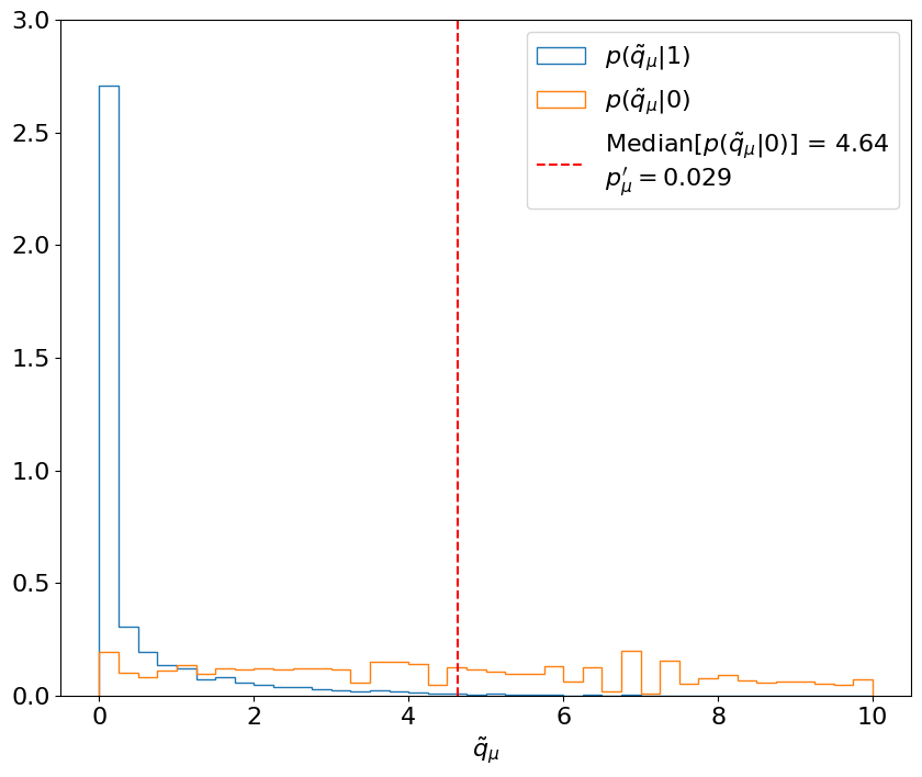
The effect of the CL criterion is demonstrated in Figure 8.14 for Examples 8.2.1 and 8.2.2. In the former, the background-only distribution is shifted to the right of the distribution. This indicates that the experiment is sensitive to and, indeed, we find . In Example 8.2.2, however, the search is not sensitive and, hence, the background-only and distributions almost completely overlap, meaning and .3
Finally, if we repeat the Neyman construction using the CL criterion instead of for Example 8.2.2, we can find an upper limit of at 95% CL, which is indeed a looser, more conservative, upper limit. The upper limit for Example 8.2.1 remains unchanged at , as we would expect.
8.2.4 Expected significances and limits
Expected significance
The focus so far has been only on evaluating the results of experiments. However, it is equally important to characterize the expected sensitivity of the experiment before running it (or before looking at the data).
Example 8.2.3. Concretely, we continue with the simple one-bin counting experiment (Section 8.2.1.). Let’s say we expect background events and — at the nominal signal strength — signal events. How do we tell if this experiment is at all useful for discovering this signal, i.e., does it have any sensitivity to the signal?
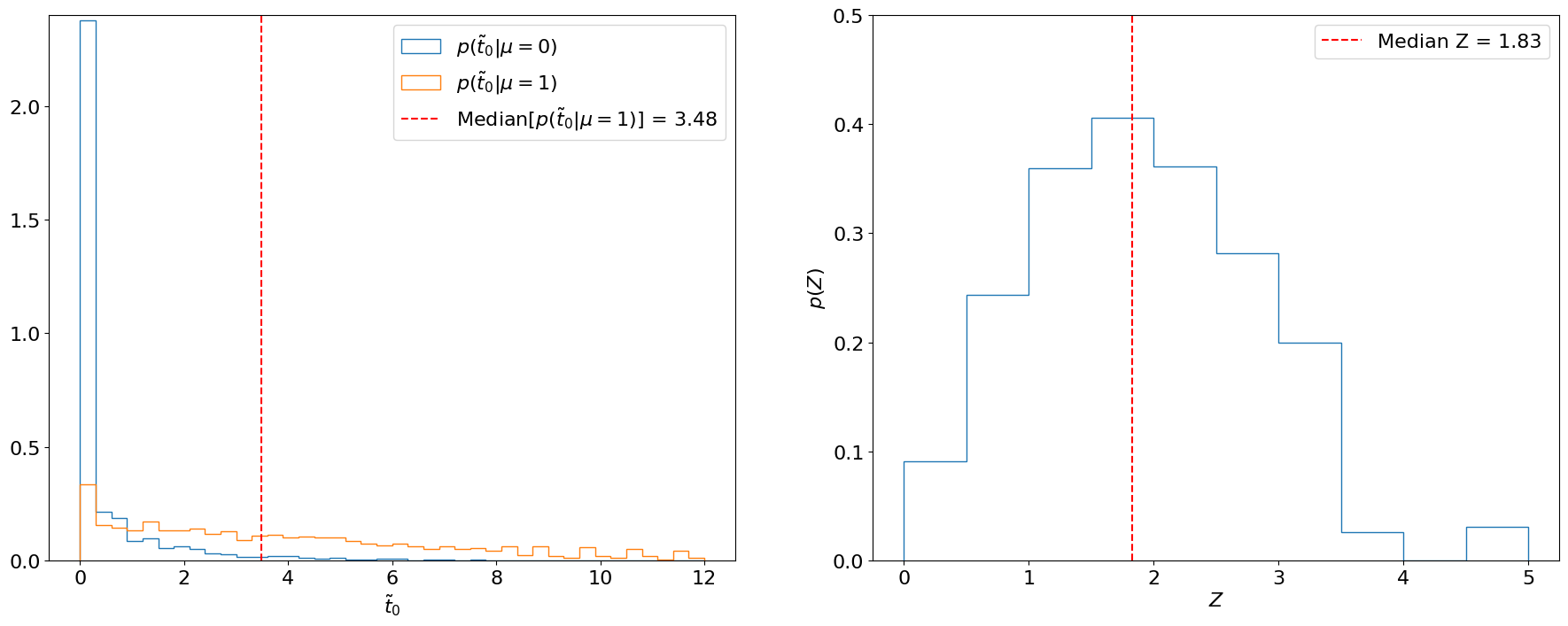
One way is to calculate the significance with which we expect to exclude the background-only hypothesis if the signal were, in fact, to exist. Practically, this means we are testing and, hence, need as before. However, now we also need the distribution of the test statistic under the background + signal hypothesis . Then, by calculating the significance for each sampled under , we can estimate the distribution of expected significances. This is illustrated for Example 8.2.3 in Figure 8.15.
Importantly, we usually quote the median of this distribution as the expected significance, since the median is “invariant” to monotonic transformations (i.e., the median -value will always correspond to the median as well, whereas the mean -value will not correspond to the mean ). Similarly, we quote the and quantiles as the and , respectively, expected significances. These quantiles correspond to the cumulative probabilities for a standard Gaussian (Figure 8.16). For Example 8.2.3, we thus find the median expected significance to be 1.83.
Note that instead of converting each sampled under into a significance and finding the median of that distribution, as in Figure 8.15 (right), we can take advantage of the invariance of the median and directly use the significance of the median under (Figure 8.15, left). We will do this below for the expected limit.
Expected limits
The other figure of merit we care about in searches is the upper exclusion limit set on the signal strength. To derive the expected limit, we do the opposite of the above and ask, if the signal were not to exist, what value of would we expect to exclude at the 95% CL.4
This means we need:
- 1.
- The distribution to solve for in Eq. 8.2.17 and be able to do the upper limit calculation (as in Section 8.2.3.);
- 2.
- to get the median (and other quantiles’) expected for different signal strengths under the background-only hypothesis; and, furthermore,
- 3.
- To scan over the different signal strengths to find the that results in a median -value of — or, rather, -value (Eq. 8.2.19), since we’re using the CL method for upper limits (Section 8.2.3.).
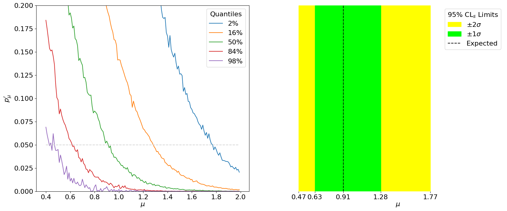
First, let’s look at the first two steps for just the signal strength in Example 8.2.3. These steps are similar to, and essentially an inversion of, the procedure for the expected significance: we’re now finding the -value with respect to the signal + background hypothesis, for the median sampled under the background-only hypothesis. This is demonstrated in Figure 8.17.
The key difference with respect to calculating the expected significance is step 3, in which this procedure has to be repeated for a range of signal strengths to find the value that gives a median (and quantile-) of . This is thus the minimum value of that we expect to be able to exclude at 95% CL, as shown in Figure 8.18.
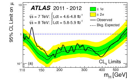
Thus, we have our expected limits. The right plot of Figure 8.18 is colloquially known as a “Brazil-band plot”, and is the standard way of representing limits. For example, Figure 8.19 is the corresponding plot by ATLAS for the Higgs discovery (scanning over the Higgs mass).
1One can find the derivation in the reference therein; essentially, like with most things in physics, this follows from Taylor expanding around the minimum...
2Ref. [301] refers to the special case of the test statistic for as .
3Note that, unlike , doesn’t follow a simple ; asymptotically, it is closer to a noncentral , as will be discussed in Section 8.3.2.
4 is the standard CL for upper limits in HEP.

