


3.2 Interactions
Like the silicon chips of more recent years, the Feynman diagram was bringing computation to the masses. — Julian Schwinger
We next make the field theory more interesting by adding interactions. We will continue with our scalar fields, first discussing the types of interactions we consider and the important concept of renormalizability in Section 3.2.1. We then focus on weakly coupled theories, where we can treat the interactions as small perturbations, as described in Section 3.2.2, and then discuss how to calculate the probability of interactions occurring using Feynman diagrams in Section 3.2.3. Finally, we outline how to translate these probabilities into the physical quantities we measure, namely decay rates and cross sections, in Section 3.2.4.
3.2.1 Interactions in the Lagrangian
Before diving into the calculations, it is useful to get an idea of the types of interactions that are “relevant” in a QFT using dimensional analysis. Consider the following generic Lagrangian for a single real scalar field:
|
| (3.2.1) |
The terms are what are new, representing interactions, and are called their coupling constants, determining their respective strengths. Broadly speaking, we only know how to make meaningful analytic calculations for interactions which we can treat as small perturbations to the free Lagrangian; indeed, there is much we do not understand about strongly-coupled theories such as QCD.
How do we decide whether an interaction is “small”? It certainly depends on the coupling constant, but is not necessarily dimensionless. The Lagrangian has energy (or mass) dimension 1 (using natural units, see Section 3.1.1), so
|
| (3.2.2) |
We need to be small relative to different things, depending on its dimension. In fact, we use its dimension (or, equivalently, that of the interaction term) to categorize different interactions.
Relevant, marginal, and irrelevant interactions
: This means must be small compared to some energy , which is typically the energy scale of our experiment or process of interest. Such an interaction therefore becomes a larger perturbation at lower energies, and smaller at high energies. These terms are called relevant because they affect the physics that we usually deal with.
: These are called marginal interactions, which are small if .
: These interactions are small at low energies and large at high energies. Because of this, we typically do not need to consider them in a QFT; hence, they are called irrelevant. Thus, in a sense, QFT is quite simple — we need only consider relevant and marginal interactions! In this case, and . The same dimensional analysis also shows why we do not consider terms with more than two derivatives.
When we do want to explore the effects of irrelevant interactions, we can parametrize them as generic operators in the Lagrangian which are suppressed by powers of , where is the energy scale at which we expect these interactions to become relevant. This is (one of) the ideas behind effective field theory (EFT) [96, 97].
Renormalizability
The types of interactions present in a theory also determine its renormalizability. Calculations in QFT are inherently plagued by infinities, one of which we encountered as the zero-point energy of the quantized free scalar field (Section B.2.2). A general method for handling ultraviolet (UV) infinities — those which arise from integrating over momenta up to — is to impose a cut-off energy scale on these integrals.
By doing so, we are essentially admitting, rightfully so, that we do not know what is going on arbitrarily high energies; hence, we do not expect our theory to be valid beyond . We then, after performing the integrals, can take the limit and hope and pray our result is independent of . This is a simplified picture of renormalization.
However, the strength of irrelevant interactions only grows with energy, so will lead to a divergence. Hence, we call theories with irrelevant interactions non-renormalizable. The SM is a renormalizable QFT and thus, as for our simple scalar field theory, its possible interactions are helpfully constrained. Most likely, it is simply an EFT of a higher energy theory, with the nonrenormalizable terms heavily suppressed by the scale of new physics!
3.2.2 S-matrix elements
As discussed above, we will focus on interactions in weakly-coupled theories, where they can be treated as small perturbations to the free Lagrangian. The quantized interaction terms comprise different combinations of creation and annihilation operators, corresponding to existing particles interacting, getting destroyed, and/or creating new ones. Broadly, we call these scattering processes, and the amplitude of these occurring is called the S-matrix element between the initial and final particles states and . The operator , for scattering, is called the S-matrix.
Note that so far we have only been discussing the abstract notion of fields in the Lagrangian. We have highlighted many connections and interpretations relating fields to physical particles, but they are not the same; fields are not particles.5 The S-matrix elements between particles are the physical quantities we measure: they are the basic observables of QFT.
Formally, fields and particles are related through the LSZ reduction formula [98], which expresses S-matrix elements in terms of the Green functions of the field (Section 3.1.4). The formula states that the S-matrix element between incoming and outgoing asymptotically free, on-shell particles is the residue of the particle pole of the associated fields’ Green functions.6
This is a very powerful result in QFT. In this section, we heuristically explain its practical consequence, which is that the S-matrix element can be calculated using the time-ordered product of the interacting fields, up to different orders in the interaction coupling constant. In the following section, we then present the even more practical method of calculating such time ordered products using Feynman diagrams.
Scalar Yukawa Lagrangian
We will use scalar Yukawa theory as an example, which couples together our real and complex scalar fields, and :
|
| (3.2.3) |
The interaction term is called a Yukawa interaction, and the weak coupling condition is .
A similar theory was originally developed by Hideki Yukawa to model the strong nuclear force between nucleons () via a hypothesized meson () [99]. Indeed, such a meson was discovered a decade later via cosmic rays, and is called the pion [100]. Nobel Prizes were awarded for both the prediction and discovery. The difference in our theory is the scalar rather than fermionic nucleon, for simplicity; we will still, however, be able to reproduce the iconic physical feature of the theory: the Yukawa potential.
Under the weak coupling condition, we can treat the interaction term as a perturbation to the free Lagrangian and use perturbation theory and the interaction picture of QM to calculate the S-matrix elements for processes at any order in (see Appendix B.3.1). For example, diagrams of first-order processes such as meson decay () and nucleon-antinucleon annihilation () are shown in Figure 3.1.


Explicit calculation yields the S-matrix element for both processes (Appendix B.3.2):
|
| (3.2.4) |
The delta function ensures momentum conservation, and is in fact a general feature of all S-matrix elements. We typically define
|
| (3.2.5) |
where is called the matrix element of the process, and is the nontrivial component we must compute. For our first-order processes, the matrix element is simply . However, explicit calculations quickly become intractable at higher orders; instead, we present a simpler alternative in the next section.
3.2.3 Feynman diagrams
Feynman diagrams are intuitive and powerful tools for calculating S-matrix elements. We have already seen examples for our first-order meson decay and nucleon-antinucleon annihilation processes in Figure 3.1. They encode a lot of information (some of which is redundant, shown only for these first diagrams for clarity) and, as we will see, directly give us the matrix elements of the processes. Feynman diagrams for higher-order processes can be constructed by adding more vertices and internal lines connecting them. Details and some conventions used in this dissertation are given in Appendix B.3.3.
Feynman rules for scalar Yukawa theory
To read off the matrix element from a Feynman diagram, we take the product of factors associated to each element of the diagram, according to the Feynman rules of the theory. These rules are ultimately derived from and encode all our information about the underlying Lagrangian. They can be written in either position or momentum space; since we are working with momentum eigenstates, we will use the latter.
Definition 3.2.1. For our scalar Yukawa theory, the Feynman rules for calculating are:7
- 1.
- Vertices:

- 2.
- Internal lines (propagators)
Mesons: Nucleons:
- 3.
- Impose momentum conservation at each vertex.
- 4.
- Integrate over the momentum flowing through each loop .
Note that the factors associated with internal lines are exactly the Feynman propagators from Section 3.1.4, which is in line with their interpretation as the amplitude for a particle to propagate from one point to another. For internal lines, the convention is for momentum to flow in the same direction as the particle flow, even for antiparticles. We see immediately that these rules reproduce the matrix element for our first-order processes, as expected. We discuss loops briefly at the end of this section; however, we focus primarily on tree-level diagrams, those without loops.
Nucleon-antinucleon scattering
One interesting higher-order example is nucleon-antinucleon scattering . At lowest order, we have the diagrams shown in Figure 3.2.


The first two Feynman rules result in the same matrix element (Eq. B.3.6) for both. Imposing momentum conservation we find:
|
| (3.2.6) |
Virtual particles
Note that by momentum conservation, the exchange meson does not have mass , as . We say that this meson is a virtual particle and is off-shell (referring to the “mass shell” in at ). This may appear dangerously unphysical; however, we are saved by the fact that such off-shell particles always appear internally in the diagram and thus can never be observed. In a sense, they can be viewed simply as a mathematical convenience in QFT; no one knows their correct physical interpretation, if any.8
Mandelstam variables
Because these types of 2-by-2 scattering processes are so common in particle physics, they have standard names, based on the momenta in the denominator of the matrix element.
Definition 3.2.2. For incoming particle momenta and and outgoing momenta and , the Mandelstam variables are defined as:
|
| (3.2.7) |
We can see that the matrix elements for nucleon-antinucelon scattering (Eq. 3.2.6) can be rewritten in terms of and as:
|
| (3.2.8) |
Hence, they are referred to as -channel and -channel diagrams, respectively. An example of a -channel diagram appears for nucleon-nucleon scattering in Figure B.2. Intuitively, is the total energy in the COM frame squared, while and are a measure of how much momentum is exchanged between the scattered particles (see Appendix B.3.3).
Resonances
Note an important point about channel diagrams: the amplitude diverges as .9 Or, in other words, as the COM energy approaches the mass of the exchanged particle (as long as ).
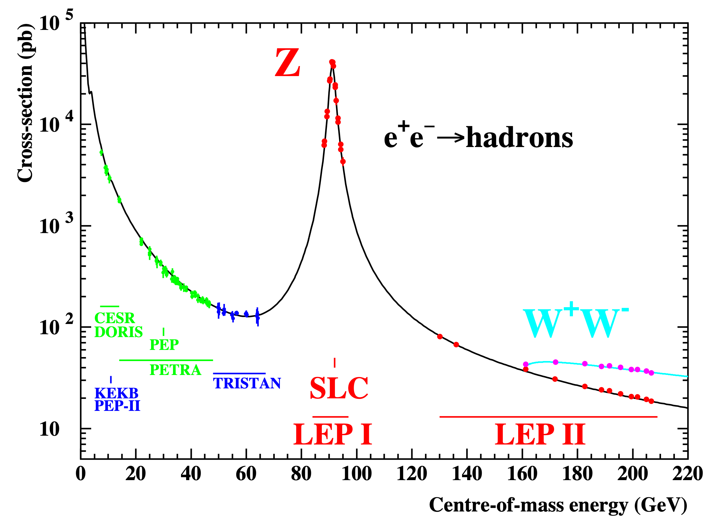
This divergence is interpreted as a resonance in the cross section (see below) of the scattering process as a function of , and allows us to discover new particles. Figure 3.3 shows a great example for hadron scattering by a series of HEP experiments with a magnificent peak at 96, the boson mass.
The classical limit and the Yukawa potential
It is important to check our QFT recovers classical physics in the appropriate limit. It will also be useful to translate the somewhat abstract idea of amplitudes to the familiar concepts of forces and potentials. We will do so by considering the nonrelativistic limit () of our above amplitudes and using the Born approximation relating the scattering amplitude between two particles to the potential between them :
|
| (3.2.9) |
where is the displacement between the particles.
First, let us consider what this potential would be classically. The static Klein-Gordon equation for a delta-function source:
|
| (3.2.10) |
can be found via the Fourier transform to be:
|
| (3.2.11) |
We can interpret this to be the profile of around a nucleon (the delta function source), and thus conversely the potential felt by another nucleon via the meson and the Yukawa interaction, under the assumption . This is entirely analogous to gauge potential in electrostatics generated by a -function source acting as the electric potential for a test charge.
Going back to our amplitude for nucleon-antinucleon scattering, the -channel diagram vanishes in the nonrelativistic limit (which essentially means it does not have a simple classical interpretation), while the -channel diagram actually stays the same:
|
| (3.2.12) |
Plugging this into the LHS of Eq. 3.2.9 and inverting the RHS integral gives us:
|
| (3.2.13) |
This is exactly the classical potential we found in Eq. 3.2.11! It is weighted by the coupling constant and to get the correct dimensions, and with a minus sign telling us potential is attractive.
Thus, we are able to reproduce Newtonian forces from the nonrelativisic limit of QFT. We also have the new interpretation of forces as simply manifestations of interactions in the Lagrangian, occurring through the exchange of virtual particles.
This potential is called the Yukawa potential, describing a force mediated by a massive boson. As expected, in the limit , we recover the familiar Coulomb potential, which is mediated by the massless photon. We can check that we obtain the same potential for nucleon-nucleon scattering and, more generally, that all forces mediated by scalars are attractive. In fact, this is true for spin-2 particles as well, which is why gravity is universally attractive! On the other hand, forces mediated by spin-1 particles, such as EM, can be either attractive or repulsive, with the charges of the particles involved determining the sign of each diagram. See e.g. Zee QFT [80] Chapter I.5 for a useful discussion.
Fourth-order diagrams and loops
So far, we have only considered tree-level diagrams, the simplest to calculate. This is in contrast to diagrams with loops, which can occur at higher order in perturbation theory. For example, at fourth-order we can have diagrams like those in Figure 3.4 for nucleon scattering.
Such diagrams contribute integrals over the loop momentum to the matrix element, which can notoriously diverge. To deal with this requires a process called renormalization, which, briefly, involves defining a cut-off energy scale for these integrals, beyond which we claim the theory is invalid. Experimentally, the main consequence is that physical parameters like the mass of particles and coupling constants in fact depend on the energy scale at which they are measured!

3.2.4 Decay rates and cross sections
In this section, we translate our S-matrix elements to physical observables: cross sections and decay rates.
Cross section
Classically for a scattering experiment, the number of particles scattered is related to the cross sectional area as:
|
| (3.2.14) |
where is the total time and is the flux of incoming particles (number of incoming particles per unit area and unit time). In QM, we define the cross section similarly, but in terms of the probability of scattering instead of :
|
| (3.2.15) |
This is a more abstract quantity in QM, but it still has units of area. The number of scattering events is related to by a factor we call the luminosity :
|
| (3.2.16) |
Here, we simply consider this the definition of luminosity, but for a collider, for example, it can be derived from the properties of the input particle beams (as will be discussed in Part II). Often, we are interested in the differential cross section with respect to kinematic variables like the solid angle or energy, so we write:
|
| (3.2.17) |
As in QM, this probability is proportional to the square of the amplitude :
|
| (3.2.18) |
where and are the normalization factors for the final and initial states (they are not equal to as discussed in Section 3.1.4), and is the differential region of final state momenta.
For the case of two incoming particles (which is what is most relevant for this dissertation), we can put all of this together to obtain the relation between differential cross section and the matrix element :
|
| (3.2.19) |
where and are the energies of the incoming particles, and are their velocities, and is called the Lorentz-invariant phase space of the final state momenta:
|
| (3.2.20) |
For the case of scattering, in the COM frame, this simplifies considerably:
|
| (3.2.21) |
and even more so when the all four masses are equal:
|
| (3.2.22) |
Decay rate
The other type of process we are interested in are decays. The decay rate is simply the probability of decay per unit time:
|
| (3.2.23) |
Using our expression for from above and simplifying, we find:
|
| (3.2.24) |
in the rest frame of the decaying particle, where is its mass. If multiple decays of the same particle are possible, we sum over the final states in the phase space integral. The total is then called the width of the particle, and is its half-life.
For our simple meson decay , we have at tree level:
|
| (3.2.25) |
where we performed the integral over (see Ref. [101] 4.2). This is in fact not too far off the expression for the decay width of the Higgs boson to fermions. What we are missing of course is that fermions are spin- particles, and we need to sum over their spin states. Fermions are described by spinor field theory, detailed in Appendix B.4.
5This point is well emphasized in Aneesh Manohar’s notes on EFT [96].
6Useful discussions of this can be found in Peskin and Schroeder [81] Chapter 7 and Schwartz [86] Chapter 6.
7These are derived nicely in Peskin and Schroeder [81] Chapter 4.7, albeit with fermionic electrons instead of our scalar “nucleons”.
8To quote Hong Liu, “In physics, when we don’t understand something, we give it a name and then claim we understand it.” [82].
9We are saved from this potential infinity by a factor to be added to the denominator due to meson decay (Tong SM [76] Chapter 3.5).