16.2 LGAE architecture

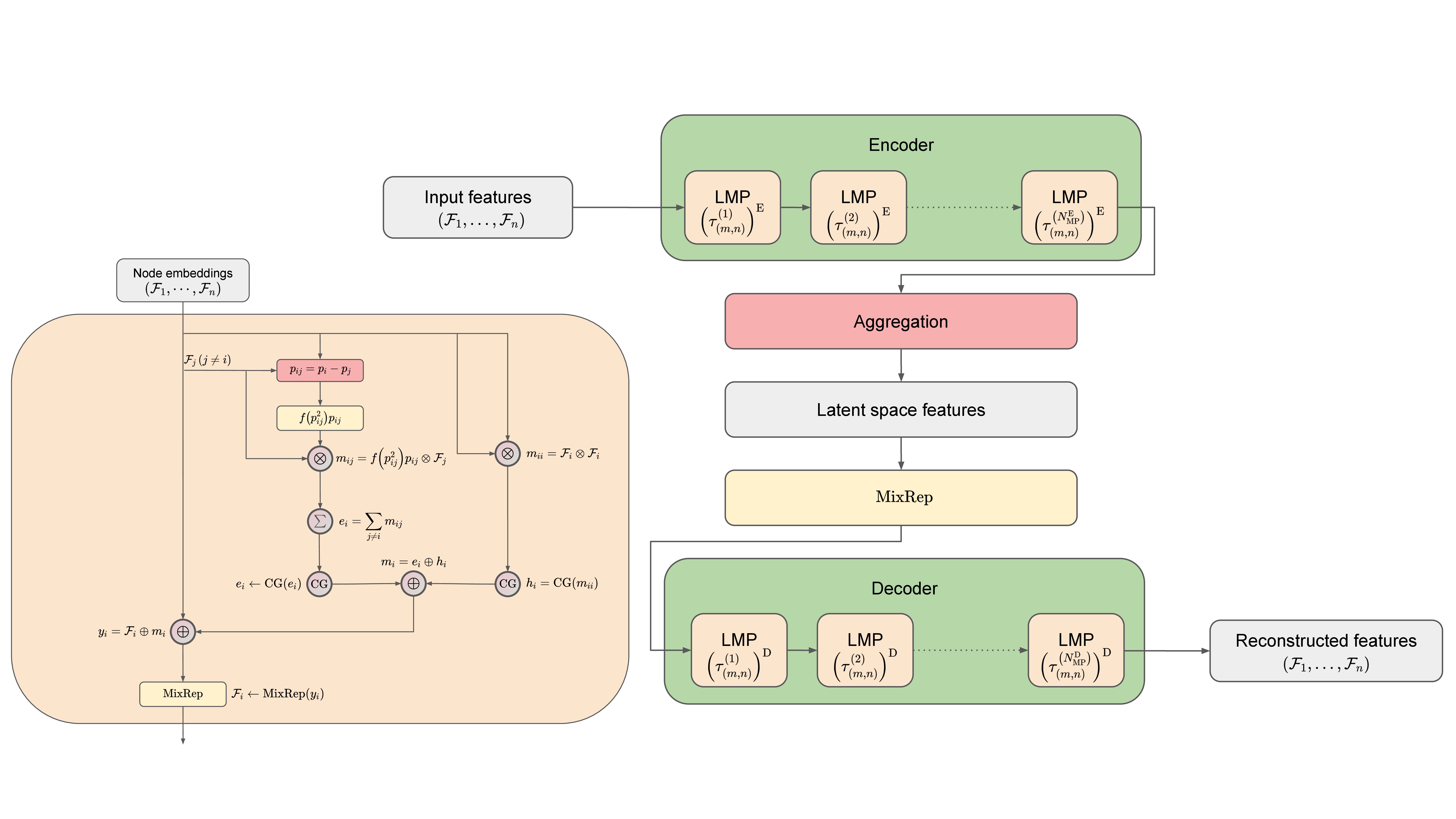
The LGAE is built out of Lorentz group-equivariant message passing (LMP) layers, which are identical to individual layers in the LGN [54]. We reinterpret them in the framework of message-passing neural networks [423], to highlight the connection to GNNs, and define them in Section 16.2.1. We then describe the encoder and decoder networks in Sections 16.2.2 and 16.2.3, respectively. The LMP layers and LGAE architecture are depicted in Figure 16.1. We provide the LGAE code, written in Python using the PyTorch ML framework [424] in Ref. [425].

16.2.1 LMP layers

LMP layers take as inputs fully-connected graphs with nodes representing particles and the Minkowski distance between respective node 4-vectors as edge features. Each node $F_i$ is defined by its features, all transforming under a corresponding irrep of the Lorentz group in the canonical basis [242], including at least one 4-vector (transforming under the $(1∕2,1∕2)$ representation) representing its 4-momentum. As in Ref [54], we denote the number of features in each node transforming under the $(m,n)$ irrep as ${\tau }_{(m,n)}$, referred to as the multiplicity of the $(m,n)$ representation.

The $(t+1)$-th MP layer operation consists of message-passing between each pair of nodes, with a message $m_{\mathit{ij}}^{(t)}$ to node $i$ from node $j$ (where $j\ne i$) and a self-interaction term $m_{\mathit{ii}}$ defined as

where $F_i^{(t)}$ are the node features of node $i$ before the $(t+1)$-th layer, $p_{\mathit{ij}}=p_i-p_j$ is the difference between node four-vectors, $p_{\mathit{ij}}^2$ is the squared Minkowski norm of $p_{\mathit{ij}}$, and $f$ is a learnable, differentiable function acting on Lorentz scalars. A Clebsch–Gordan (CG) decomposition, which reduces the features to direct sums of irreps of ${\mathrm{SO}}^{+}(3,1)$, is performed on both terms before concatenating them to produce the message $m_i$ for node $i$:

where the summation over the destination node $j$ ensures permutation symmetry because it treats all other nodes equally.

Finally, this aggregated message is used to update each node’s features, such that

for all $i\in \{1,\dots ,N_{\mathrm{particle}}\}$, where $W^{(t+1)}$ is a learnable node-wise operator which acts as separate fully-connected linear layers $W_{(m,n)}^{(t+1)}$ on the set of components living within each separate $(m,n)$ representation space, outputting a chosen ${\tau }_{(m,n)}^{(t+1)}$ number of components per representation. In practice, we then truncate the irreps to a maximum dimension to make computations more tractable.

16.2.2 Encoder

The encoder takes as input an $N$-particle cloud, where each particle is each associated with a 4-momentum vector and an arbitrary number of scalars representing physical features such as mass, charge, and spin. Each isotypic component is initially transformed to a chosen multiplicity of ${\left({\tau }_{(m,n)}^{(0)}\right)}_E$ via a node-wise operator $W^{(0)}$ identical conceptually to $W^{(t+1)}$ in Eq. (16.2.4). The resultant graph is then processed through $N_{\mathrm{MP}}^E$ LMP layers, specified by a sequence of multiplicities ${\left\{{\left({\tau }_{(m,n)}^{(t)}\right)}_E\right\}}_{t=1}^{N_{\mathrm{MP}}^E}$, where ${\left({\tau }_{(m,n)}^{(t)}\right)}_E$ is the multiplicity of the $(m,n)$ representation at the $t$-th layer. Weights are shared across the nodes in a layer to ensure permutation equivariance. After the final MP layer, node features are aggregated to the latent space by a component-wise minimum (min), maximum (max), or mean. The min and max operations are performed on the respective Lorentz invariants. We also find, empirically, interesting performance by simply concatenating isotypic components across each particle and linearly “mixing" them via a learned matrix as in Eq. (16.2.4). Crucially, unlike in Eq. (16.2.4), where this operation only happens per particle, the concatenation across the particles imposes an ordering and, hence, breaks the permutation symmetry.

16.2.3 Decoder

The decoder recovers the $N$-particle cloud by acting on the latent space with $N$ independent, learned linear operators, which again mix components living in the same representations. This cloud passes through $N_{\mathrm{MP}}^D$ LMP layers, specified by a sequence of multiplicities ${\left\{{\left({\tau }_{(m,n)}^{(t)}\right)}_D\right\}}_{t=1}^{N_{\mathrm{MP}}^D}$, where ${\left({\tau }_{(m,n)}^{(t)}\right)}_D$ is the multiplicity of the $(m,n)$ representation at the $t$-th LMP layer. After the LMP layers, node features are mixed back to the input representation space ${\left(D^{(0,0)}\right)}^{\oplus {\tau }_{(0,0)}^{(0)}}\oplus D^{(1∕2,1∕2)}$ by applying a linear mixing layer and then truncating other isotypic components.