16.3 Experiments

We experiment with and evaluate the performance of the LGAE and baseline models on reconstruction and anomaly detection for simulated high-momentum jets from the JetNet dataset. In this section, we describe the dataset in more detail in Section 16.3.1, the different models we consider in Section 16.3.2, the reconstruction and anomaly detection results in Sections 16.3.3 and 16.3.4 respectively, an interpretation of the LGAE latent space in Section 16.3.5, and finally experiments of the data efficiency of the different models in Section 16.3.6.

16.3.1 Dataset

We use 30-particle high $p_T$ jets from the JetNet dataset as described in Chapter 9.2, obtained using the JetNet library from Chapter 15. The model is trained on jets produced from gluons and light quarks, which are collectively referred to as quantum chromodynamics (QCD) jets.

As before, we represent the jets as a point cloud of particles, termed a “particle cloud”, with the respective 3-momenta, in absolute coordinates, as particle features. In the processing step, each 3-momentum is converted to a 4-momentum: $p^{\mu }=(|p|,p)$, where we consider the mass of each particle to be negligible. We use a $60\%∕20\%∕20\%$ training/testing/validation splitting for the total 177,000 jets. For evaluating performance in anomaly detection, we consider jets from JetNet produced by top quarks, $W$ bosons, and $Z$ bosons as our anomalous signals.

We note that the detector and reconstruction effects in JetNet, and indeed in real data collected at the LHC, break the Lorentz symmetry; hence, Lorentz equivariance is generally an approximate rather than an exact symmetry of HEP data. We assume henceforth that the magnitude of the symmetry breaking is small enough that imposing exact Lorentz equivariance in the LGAE is still advantageous — and the high performance of the LGAE and classification models such as LorentzNet support this assumption. Nevertheless, important studies in future work may include quantifying this symmetry breaking and considering approximate symmetries in NNs.

16.3.2 Models

LGAE model results are presented using both the min-max (LGAE-Min-Max) and “mix” (LGAE-Mix) aggregation schemes for the latent space, which consists of varying numbers of complex Lorentz vectors — corresponding to different compression rates. We compare the LGAE to baseline GNN and CNN autoencoder models, referred to as “GNNAE” and “CNNAE” respectively.

The GNNAE model is composed of fully-connected MPNNs adapted from MPGAN (Section 10.1). We experiment with two types of encodings: (1) particle-level (GNNAE-PL), as in the PGAE [67] model, which compresses the features per node in the graph but retains the graph structure in the latent space, and (2) jet-level (GNNAE-JL), which averages the features across each node to form the latent space, as in the LGAE. Particle-level encodings produce better performance overall for the GNNAE, but the jet-level provides a more fair comparison with the LGAE, which uses jet-level encoding to achieve a high level of compression of the features.

For the CNNAE, which is adapted from Ref. [248], the relative coordinates of each input jets’ particle constituents are first discretized into a $40\times 40$ grid. The particles are then represented as pixels in an image, with intensities corresponding to $p_T^{\mathrm{rel}}$. Multiple particles per jet may correspond to the same pixel, in which case their $p_T^{\mathrm{rel}}$’s are summed. The CNNAE has neither Lorentz nor permutation symmetry, however, it does have in-built translation equivariance in $\eta -\varphi$ space.

Hyperparameter and training details for all models can be found in E.1 and E.2, respectively, and a summary of the relevant symmetries respected by each model is provided in Table 16.1. The LGAE models are verified to be equivariant to Lorentz boosts and rotations up to numerical error, with details provided in E.3.

16.3.3 Reconstruction

We evaluate the performance of the LGAE, GNNAE, and CNNAE models, with the different aggregation schemes discussed, on the reconstruction of the particle and jet features of QCD jets. We consider relative transverse momentum $p_T^{\mathrm{rel}}=p_T^{\mathrm{particle}}∕p_T^{\mathrm{jet}}$ and relative angular coordinates ${\eta }^{\mathrm{rel}}={\eta }^{\mathrm{particle}}-{\eta }^{\mathrm{jet}}$ and ${\varphi }^{\mathrm{rel}}={\varphi }^{\mathrm{particle}}-{\varphi }^{\mathrm{jet}}(\mathit{mod}2\pi )$ as each particle’s features, and total jet mass, $p_T$ and $\eta$ as jet features. We define the compression rate as the ratio between the total dimension of the latent space and the number of features in the input space: $30\mathrm{particles}\times 3\mathrm{features}\mathrm{per}\mathrm{particle}=90$.

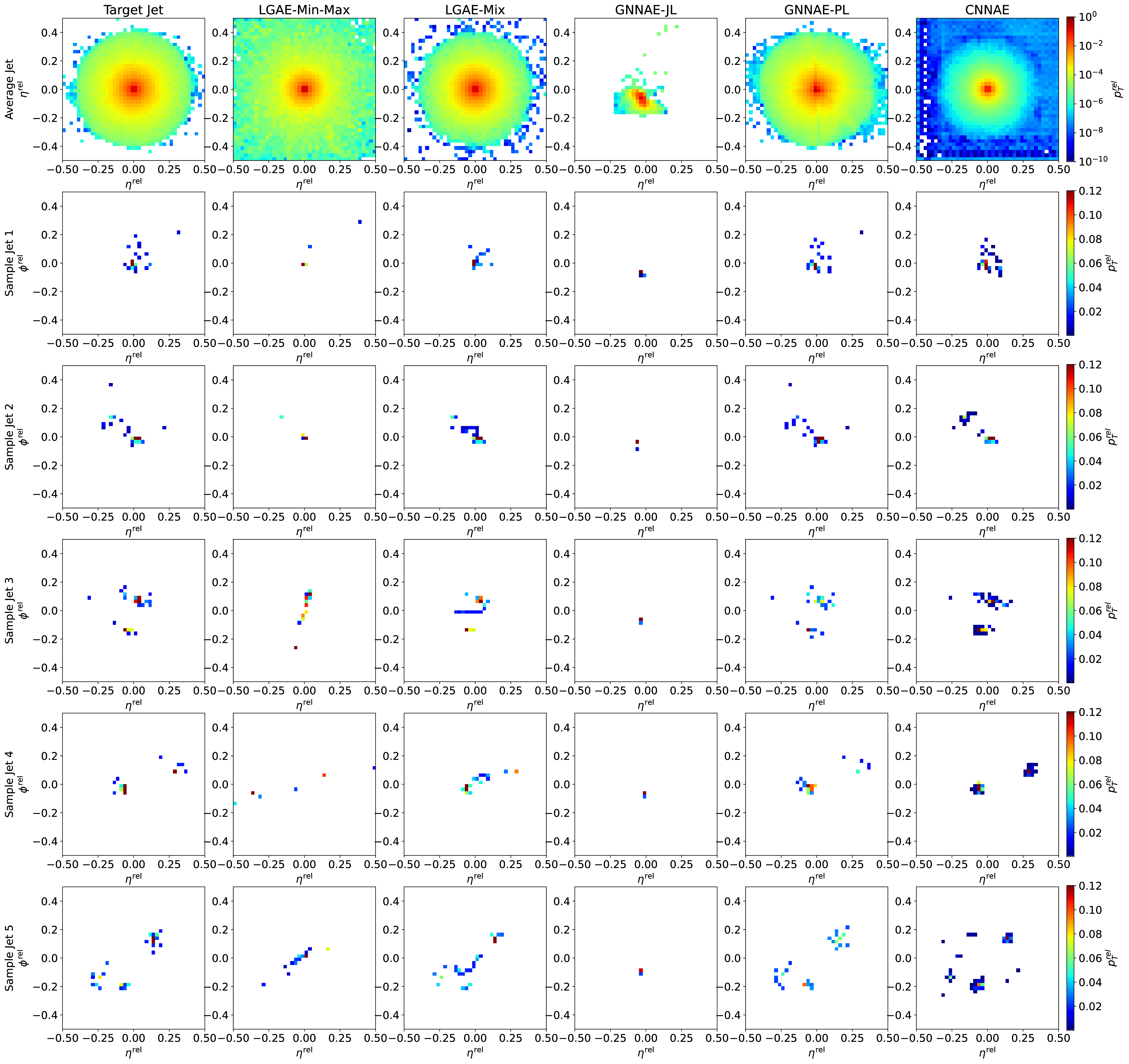
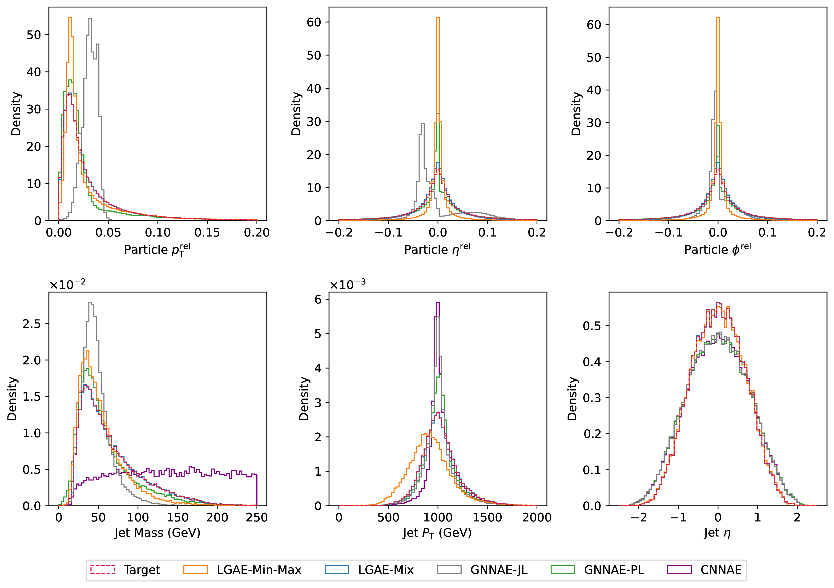
Figure 16.2 shows random samples of jets, represented as discrete images in the angular-coordinate plane, reconstructed by the models with similar levels of compression in comparison to the true jets. Figure 16.3 shows histograms of the reconstructed features compared to the true distributions. The differences between the two distributions are quantified in Table 16.2 by calculating the median and interquartile ranges (IQR) of the relative errors between the reconstructed and true features. To calculate the relative errors of particle features for the permutation invariant LGAE and GNNAE models, particles are matched between the input and output clouds using the Jonker–Volgenant algorithm [303, 426] based on the L2 distance between particle features. Due to the discretization of the inputs to the CNNAE, reconstructing individual particle features is not possible; instead, only jet features are shown.¹

We can observe visually in Figure 16.2 that out of the two permutation invariant models, while neither is able to reconstruct the jet substructure perfectly, the LGAE-Min-Max outperforms the GNNAE-JL. Perhaps surprisingly, the permutation-symmetry-breaking mix aggregation scheme improves the LGAE in this regard. Both visually in Figure 16.3 and quantitatively from Tables 16.2 and 16.3, we conclude that the LGAE-Mix has the best performance overall, significantly outperforming the GNNAE and CNNAE models at similar compression rates. The LGAE-Min-Max model outperforms the GNNAE-JL in reconstructing all features and the GNNAE-PL in all but the IQR of the particle angular coordinates.

16.3.4 Anomaly detection

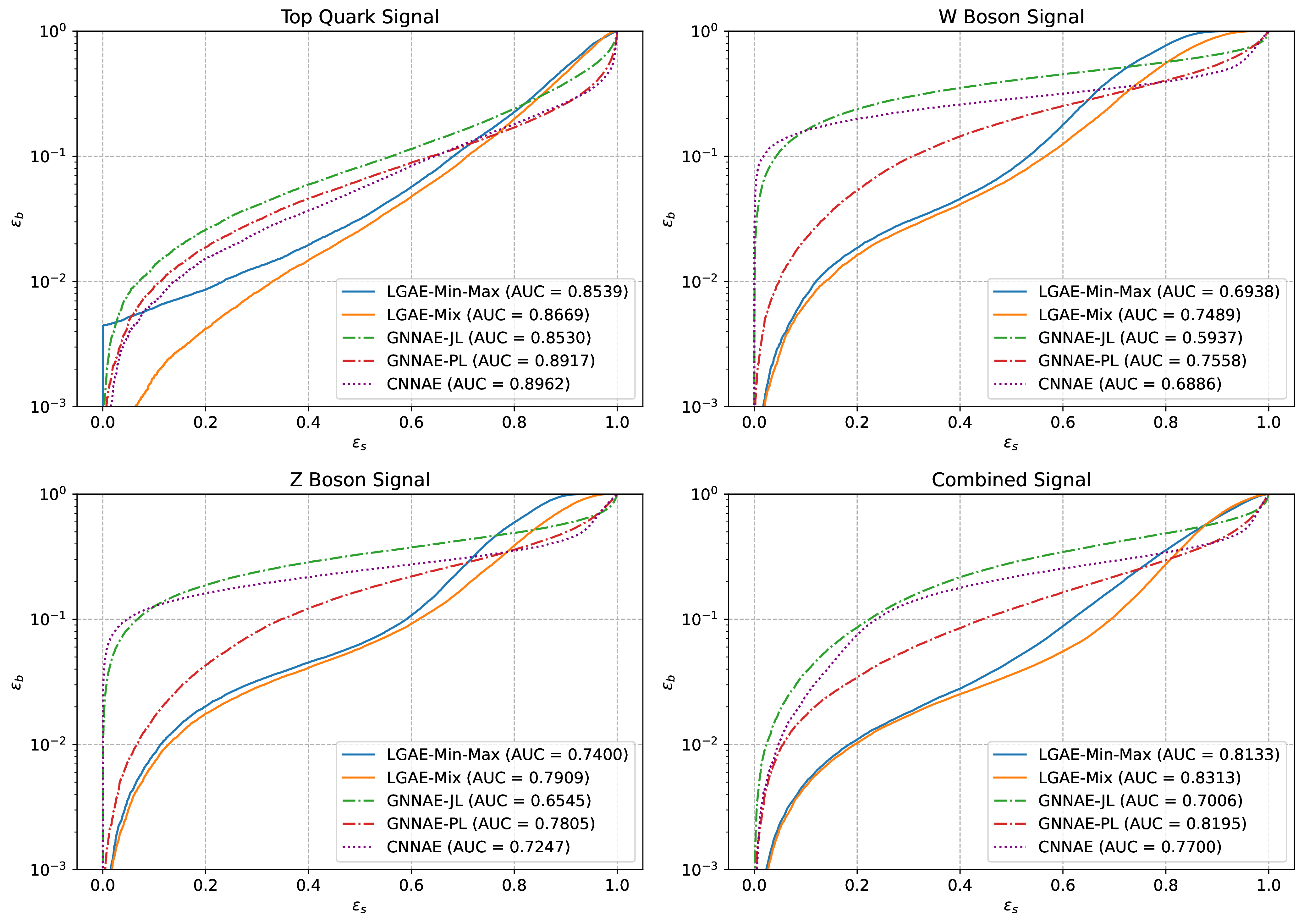
We test the performance of all models as unsupervised anomaly detection algorithms by pre-training them solely on QCD and then using the reconstruction error for the QCD and new signal jets as the discriminating variable. We consider top quark, $\mathrm{\text{W}}$ boson, and $\mathrm{\text{Z}}$ boson jets as potential signals and QCD as the “background”. We test the Chamfer distance, energy mover’s distance [325] — the earth mover’s distance applied to particle clouds, and MSE between input and output jets as reconstruction errors, and find the Chamfer distance most performant for all graph-based models. For the CNNAE, we use the MSE between the input and reconstructed image as the anomaly score.

Receiver operating characteristic (ROC) curves showing the signal efficiencies (${𝜀}_s$) versus background efficiencies (${𝜀}_b$) for individual and combined signals are shown in Figure 16.4,² and ${𝜀}_s$ values at particular background efficiencies are given in Table 16.4. We see that in general the permutation equivariant LGAE and GNNAE models outperform the CNNAE, strengthening the case for considering equivariance in neural networks. Furthermore, LGAE models have significantly higher signal efficiencies than GNNAEs and CNNAEs for all signals when rejecting $>90\%$ of the background (which is the minimum level we typically require in HEP), and LGAE-Mix consistently performs better than LGAE-Min-Max.

16.3.5 Latent space interpretation

The outputs of the LGAE encoder are irreducible representations of the Lorentz groups; they consist of a pre-specified number of Lorentz scalars, vectors, and potentially higher-order representations. This implies a significantly more interpretable latent representation of the jets than traditional autoencoders, as the information distributed across the latent space is now disentangled between the different irreps of the Lorentz group. For example, scalar quantities like the jet mass will necessarily be encoded in the scalars of the latent space, and jet and particle 4-momenta in the vectors.

We demonstrate the latter empirically on the LGAE-Mix model (${\tau }_{(1∕2,1∕2)}=2$) by looking at correlations between jet 4-momenta and the components of different combinations of latent vector components. Figure 16.5 shows that, in fact, the jet momenta is encoded in the imaginary component of the sum of the latent vectors.

We can also attempt to understand the anomaly detection performance by looking at the encodings of the training data compared to the anomalous signal. Figure 16.6 shows the individual and total invariant mass of the latent vectors of sample LGAE models for QCD and top quark, W boson, and Z boson inputs. We observe that despite the overall similar kinematic properties of the different jet classes, the distributions for the QCD background are significantly different from the signals, indicating that the LGAE learns and encodes the difference in jet substructure — despite substructure observables such as jet mass not being direct inputs to the network — explaining the high performance in anomaly detection.

Finally, while in this section we showcased simple “brute-force” techniques for interpretability by looking directly at the distributions and correlations of latent features, we hypothesize that such an equivariant latent space would also lend itself effectively to the vast array of existing explainable AI algorithms [427, 428], which generically evaluate the contribution of different input and intermediate neuron features to network outputs. We leave a detailed study of this to future work.

16.3.6 Data efficiency

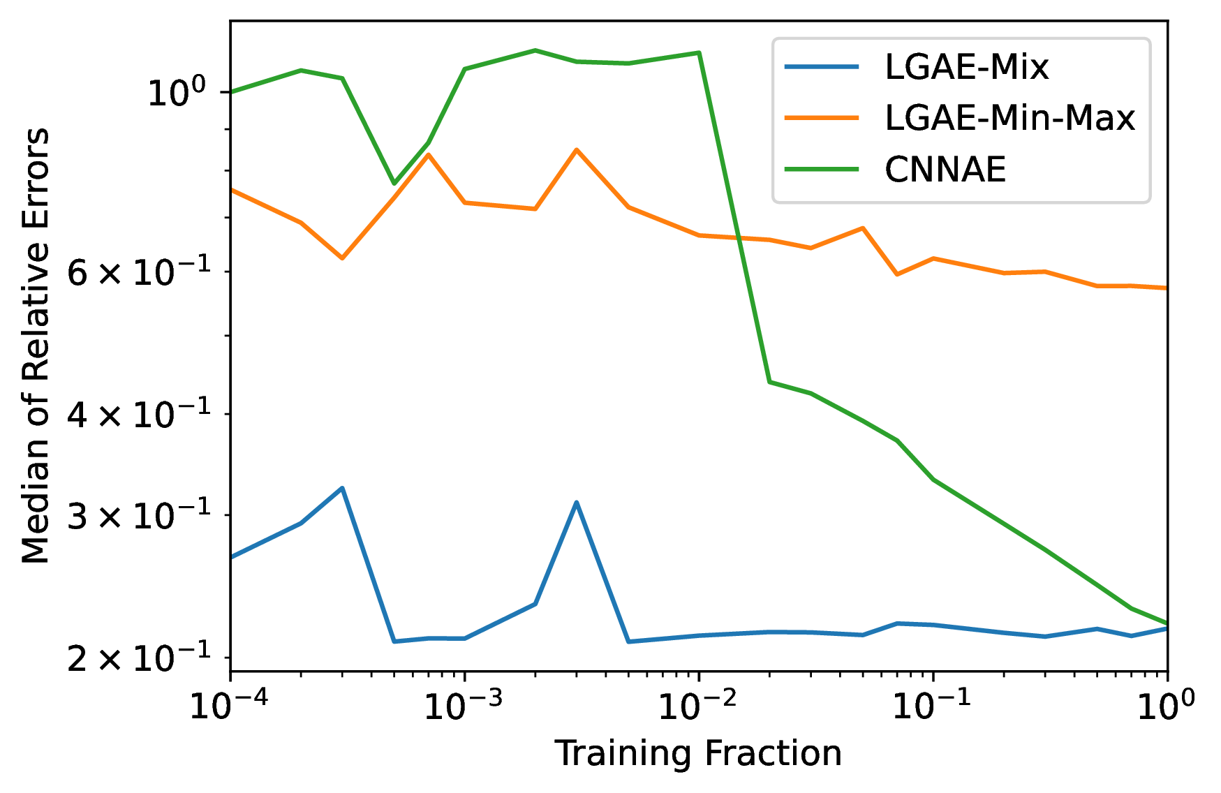
In principle, equivariant neural networks should require less training data for high performance, since critical biases of the data, which would otherwise have to be learned by non-equivariant networks, are already built in. We test this claim by measuring the performances of the best-performing LGAE and CNNAE architectures from Section 16.3.3 trained on varying fractions of the training data.

The median magnitude of the relative errors between the reconstructed and true jet masses of the different models and fractions is shown in Figure 16.7. Each model is trained five times per training fraction, with different random seeds, and evaluated on the same-sized validation dataset; the median of the five models is plotted. We observe that, in agreement with our hypothesis, the LGAE models both maintain their high performance all the way down to training on 1% of the data, while the CNNAE’s performance steadily degrades down to 2% and then experiences a further sharp drop.