Introduction to Likelihoods and Test Statistics

2. Introduction to Likelihoods and Test Statistics#

2.1. The data model#

Let’s take the simplest possible case of a (one bin) counting experiment, where in our “signal region” we expect $s$ signal events and $b$ background events. The probability to observe $n$ events in our signal region is distributed as a Poisson with mean $s+b$:

(2.1)#\[P(n; s, b) = Pois(n; s+b) = \frac{(s+b)^n e^{-(s+b)}}{n!}\]

Since we have only one observation but two free parameters, this experiment is underconstrained. So, let’s also add a “control region” where we expect no signal and $b$ background events. The probability to observe $m$ events in our control region is therefore:

(2.2)#\[Pois(m; b) = \frac{b^m e^{-b}}{m!}\]

Combining the two, the joint probability distribution for $n$ and $m$ is:

(2.3)#\[P(n, m; s, b) = Pois(n; s+b) \cdot Pois(m; b) = \frac{(s+b)^n e^{-(s+b)}}{n!} \cdot \frac{b^m e^{-b}}{m!}\]

This is also called the model for the data.

2.2. The likelihood function#

In the frequentist philosophy, however, all our parameters $n$, $m$ etc. are simply fixed values of nature and, hence, don’t have a probability distribution. Instead we work with the likelihood function of our parameters of interest ($s$) and “nuisance parameters” ($b$), given fixed values for $n$ and $m$:

(2.4)#\[L(s, b) = P(n, m; s, b) = \frac{(s+b)^n e^{-(s+b)}}{n!} \cdot \frac{b^m e^{-b}}{m!}.\]

Importantly, this is not a probability distribution on $s$ and $b$! To derive that, we would have to use Bayes’ rule to go from $P(n, m; s, b) \to P(s, b; n, m)$; however, such probability distributions don’t make sense in our frequentist world view, so we’re stuck with this likelihood ~~nonsense~~ formulation. For a better explanation of this, I recommend Section 2 in Ref. [2] regarding frequentist vs Bayesian reasoning. I also like Nick Smith’s quote, “Everyone’s a Bayesian in their head, but we use frequentist probability in HEP because we can’t agree on a prior.”

Often, it’s more convenient to consider the negative log-likelihood:

(2.5)#\[-\ln L = \ln n! + \ln m! + s + 2b - n\ln(s+b) - m \ln b\]

2.3. The profile likelihood ratio#

The goal of any experiment is to test the compatibility of the observed data ($n, m$ here) with a certain hypothesis $H$. We do this by mapping the data to a “test statistic” $t$, which is just a number, and comparing it against its distribution under $H$, $P(t| H)$. The problem, thus, boils down to 1) choosing the most effective $t$ for testing $H$, and 2) obtaining $P(t| H)$.

In the case of testing a particular signal strength, we typically consider the “profile likelihood ratio”:

(2.6)#\[\lambda(s) = \frac{L(s, \hat{\hat{b}}(s))}{L(\hat{s}, \hat{b})},\]

where $\hat{s}, \hat{b}$ are the maximum-likelihood estimates (MLEs) for $s$ and $b$, given the observations $n, m$, and $\hat{\hat{b}}(s)$ is the MLE for $b$ given $n, m$, and $s$. The MLE for a parameter is simply the value of it for which the likelihood is maximized, and will be discussed in the next section. The numerator of $\lambda(s)$ can be thought of as a way to ``marginalize’’ over the nuisance parameters by simply values that maximize the likelihood for any given $s$, while the denominator is effectively a normalization factor, such that $\lambda(s) \leq 1$.

Again, it’s often more convenient to use the (negative) logarithm:

(2.7)#\[t_s = -2 \ln \lambda(s)\]

This statistic also has nice asymptotic forms, which we’ll see later.

2.4. Maximum-likelihood estimates#

MLEs for $s$ and $b$ can be found for this example by setting the derivative of the negative log-likelihood to 0 (more generally, this would require numerical minimization):

(2.8)#\[\begin{split}\frac{\partial (-\ln L)}{\partial s} &= 1 - \frac{n}{s+b} = 0 \\ \frac{\partial (-\ln L)}{\partial b} &= 2 - \frac{n}{s+b} - \frac{m}{b} = 0\end{split}\]

Solving simultaneously yields, as you might expect:

(2.9)#\[\hat{b} = m, \hat{s} = n - m,\]

Or just for $\hat{\hat{b}}(s)$ from Eq. (2.8):

(2.10)#\[2b^2 + (2s - n - m)b - ms = 0\]

Plugging this back in, we can get $\lambda(s)$ and $t_s$ for any given $s$ (which I won’t write out because even in this simple example they’re painful).

The next step would be to derive $P(t| H)$, by either sampling $t$s for multiple “toy” generated events or using an asymptotic (i.e., large $n,m$) approximation.

For now, however, let’s pause here and code up what we have so far to get a sense of what this all looks like.

import numpy as np
import matplotlib as mpl
import matplotlib.pyplot as plt
from scipy.special import factorial

2.5. Define and plot our model#

def poisson(n, mu):
    return np.exp(-mu) * np.power(mu, n) / factorial(n)


def model(n, m, s, b):
    return poisson(n, s + b) * poisson(m, b)

sbs = [(10.0, 1.0), (1.0, 10.0), (5.0, 5.0)]  # sample (s, b) values

ns, ms = np.meshgrid(np.arange(1, 16), np.arange(1, 16))
fig, ax = plt.subplots(1, len(sbs), figsize=(5.4 * len(sbs), 4))
for i, (s, b) in enumerate(sbs):
    im = ax[i].pcolormesh(
        ms, ns, model(ns, ms, s, b), cmap="turbo", norm=mpl.colors.LogNorm(vmax=1)
    )
    ax[i].set_title(rf"$s = {s}, b = {b}$")
    ax[i].set_xlabel(r"$m$")
    ax[i].set_ylabel(r"$n$")
fig.colorbar(im, ax=ax.ravel().tolist(), pad=0.01, label="Probability")
plt.show()

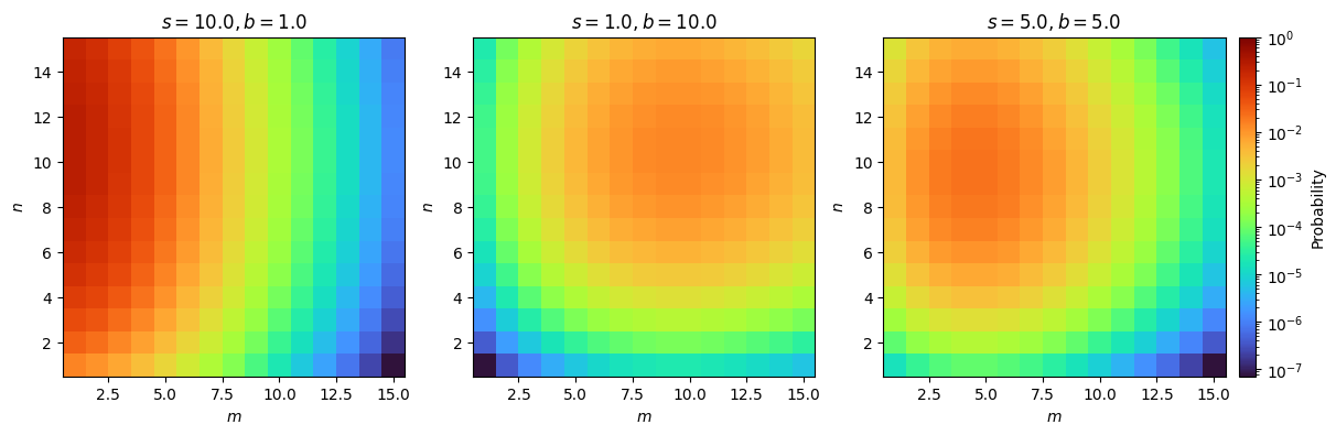
_images/07ad5e45b3525abc746c1ecf435c1467684c23be5ce03ed8469edabf56005090.png — Fig. 2.1 Our probability model.#

Standard 2D Poisson distributions.

2.6. Define and plot the profile likelihood ratio and $t_s$ test statistic#

def poisson_nofactorial(n, mu):
    """
    In likelihood ratios the factorials in denominators cancel out,
    so they're removed here to make computations faster
    """
    return np.exp(-mu) * np.power(mu, n)


def log_poisson_nofactorial(n, mu):
    return -mu + n * np.log(mu)


def likelihood_nofactorial(s, b, n, m):
    return poisson_nofactorial(n, s + b) * poisson_nofactorial(m, b)


def log_likelihood_nofactorial(s, b, n, m):
    return log_poisson_nofactorial(n, s + b) + log_poisson_nofactorial(m, b)


def shat(n, m):
    return n - m


def bhat(n, m):
    return m


def bhathat(s, n, m):
    """Using the quadratic formula and only the positive solution"""
    return ((n + m - 2 * s) + np.sqrt((n + m - 2 * s) ** 2 + 8 * s * m)) / 4


def lambda_s(s, n, m, b=None):
    """Profile likelihood ratio, b can optionally be fixed (for demo below)"""
    bhh, bh = (bhathat(s, n, m), bhat(n, m)) if b is None else (b, b)
    return likelihood_nofactorial(s, bhh, n, m) / likelihood_nofactorial(shat(n, m), bh, n, m)


def t_s(s, n, m, b=None):
    """-2ln(lambda), b can optionally be fixed (for demo below)"""
    bhh, bh = (bhathat(s, n, m), bhat(n, m)) if b is None else (b, b)
    return -2 * (
        log_likelihood_nofactorial(s, bhh, n, m) - log_likelihood_nofactorial(shat(n, m), bh, n, m)
    )

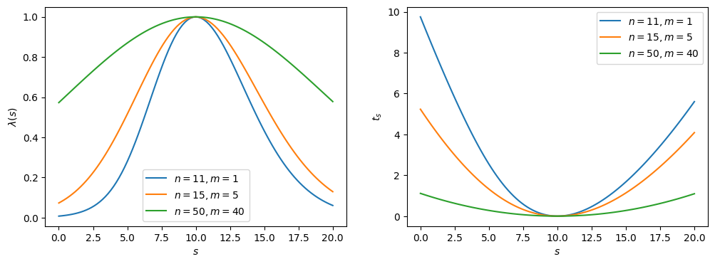
Fig. 2.2 Likelihood ratio $\lambda$ and test statistic $t_s$.#

The maximum (minimum) of the profile likelihood ratio ($t_s$) is at $s = n - m = 10$, as we expect; however, as the ratio between $n$ and $m$ decreases — i.e., the experiment becomes more noisy — the distributions broaden, representing the reduction in sensitivity, or the higher uncertainty on the true value of $s$.

Note

Note that the likelihood ratio and $t_s$ are broader due to the nuisance parameter; i.e., because we are missing information about $b$. This can be demonstrated explicitly by re-making these plots with $b$ fixed to $m$ (emulating perfect information of $b$).

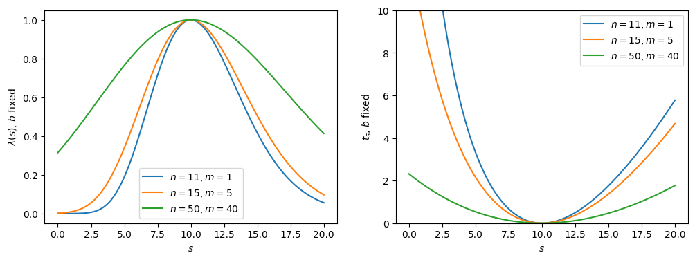
Fig. 2.3 Likelihood ratio and test statistic with fixed $b$.#

Indeed, the functions are narrower with perfect knowledge of $b$. More generally, increasing (decreasing) the uncertainties on the nuisance parameters will broaden (narrow) the test statistic distribution. This is which is why experimentally we want to constrain them through auxiliary measurements as much as possible.

2.7. Alternative test statistic#

So far, our construction allows for $s < 0$; however, physically the number of signal events can’t be negative. Rather than incorporating this constraint the model, it’s more convenient to impose this is in the test statistic, by defining:

(2.11)#\[\begin{split} \tilde{\lambda}(s) = \left\{ \begin{array}{ll} \frac{L(s, \hat{\hat{b}}(s))}{L(\hat{s}, \hat{b})}, & \mbox{$\hat{s}\geq0$}.\\ \frac{L(s, \hat{\hat{b}}(s))}{L(\hat{0}, \hat{\hat{b}}(0))}, & \mbox{$\hat{s}<0$}. \end{array} \right., \end{split}\]

and

(2.12)#\[ \tilde{t}_s = -2\ln \tilde{\lambda}(s) \]

This is what it looks like:

def lambda_zero_s(s, n, m):
    """Alternative lambda when shat < 0"""
    return likelihood_nofactorial(s, bhathat(s, n, m), n, m) / likelihood_nofactorial(
        0, bhathat(0, n, m), n, m
    )


def lambda_tilde_s(s, n, m):
    s, n, m = [np.array(x) for x in (s, n, m)]  # convert to numpy arrays
    bhh, bh, sh = bhathat(s, n, m), bhat(n, m), shat(n, m)
    neg_shat_mask = sh < 0  # find when s^ is < 0
    lam_s = lambda_s(s, n, m)
    lam_zero = lambda_zero_s(s, n, m)
    # replace values where s^ < 0 with lam_zero
    lam_s[neg_shat_mask] = lam_zero[neg_shat_mask]
    return lam_s


def t_zero_s(s, n, m):
    """Alternative test statistic when shat < 0"""
    return -2 * (
        log_likelihood_nofactorial(s, bhathat(s, n, m), n, m)
        - log_likelihood_nofactorial(0, bhathat(0, n, m), n, m)
    )


def t_tilde_s(s, n, m):
    s, n, m = [np.array(x) for x in (s, n, m)]  # convert to numpy arrays
    bhh, bh, sh = bhathat(s, n, m), bhat(n, m), shat(n, m)
    neg_shat_mask = sh < 0  # find when s^ is < 0
    ts = t_s(s, n, m)
    t_zero = t_zero_s(s, n, m)
    # replace values where s^ < 0 with lam_zero
    ts[neg_shat_mask] = t_zero[neg_shat_mask]
    return ts

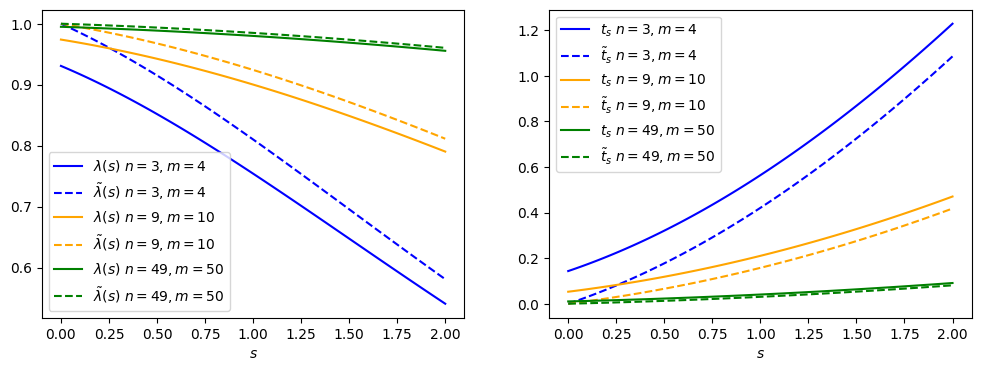
_images/b8fe670aa176da4d4a7f1c173a3f5fdb0a1956927c3082001a8f4799617d7ccd.png — Fig. 2.4 Comparing the nominal vs alternative test statistic.#

The $\tilde{\lambda}(s) = 1$ and $\tilde{t}_s = 0$ values are now at $s = 0$, since physically that is what fits best with our data (even though the math says otherwise.)

2.8. Summary#

We walked through defining a probability model for the data, the associated likelihood function, and the behaviour of common test statistics. In Chapter 3, I will go over using this for hypothesis testing.

Introduction to Likelihoods and Test Statistics

Contents