Hypothesis Testing and Discovery Significance

3. Hypothesis Testing and Discovery Significance#

3.1. Recap#

We defined our probability model and likelihood function for a simple one bin counting experiment with $n$ events, $s$ signal and $b$ background, in our signal region and $m$ events, $b$ background, in our control region:

(3.1)#\[ P(n, m; s, b) = \frac{(s+b)^n e^{-(s+b)}}{n!} \cdot \frac{b^m e^{-b}}{m!} = L(s, b), \]

and our test statistic $\tilde{t}_s$:

(3.2)#\[\begin{split} \tilde{\lambda}(s) = \left\{ \begin{array}{ll} \frac{L(s, \hat{\hat{b}}(s))}{L(\hat{s}, \hat{b})}, & \mbox{$\hat{s}\geq0$}.\\ \frac{L(s, \hat{\hat{b}}(s))}{L(0, \hat{\hat{b}}(0))}, & \mbox{$\hat{s}<0$}. \end{array} \right., \quad \tilde{t}_s=-2\ln \tilde{\lambda}(s), \end{split}\]

and solved for $\hat{s}, \hat{b}, \hat{\hat{b}}(s)$ for given $n, m$ to find an analytic form for $\tilde{t}_s$.

Next, we want to translate this to a probability distribution of $\tilde{t}_s$ under a particular signal hypothesis ($H_s$) (i.e., an assumed value of $s$): $p(\tilde{t}_s|H_s)$, or just $p(\tilde{t}_s|s)$ for simplicity.

3.2. Hypothesis testing#

The goal of any experiment is to test whether our data support or exclude a particular hypothesis $H$, and quantify the (dis)agreement. For example, to what degree did our search for the Higgs boson agree or disagree with the standard model hypothesis?

We have already discussed the process of mapping our data to a scalar test statistic $t$ that we can use to test $H$. However, we need to know the probability distribution of $t$ under $H$ to quantify the (in)consistency of the observed data with $H$ and decide whether or not to exclude $H$.

We also recognize that there’s always a chance that we will exclude $H$ even if it’s true (called a Type I error, or a false positive), or not exclude $H$ when it’s false (Type II error, or false negative). The probability of each is referred to as $\alpha$ and $\beta$, respectively. See this handy table from Wikipedia:

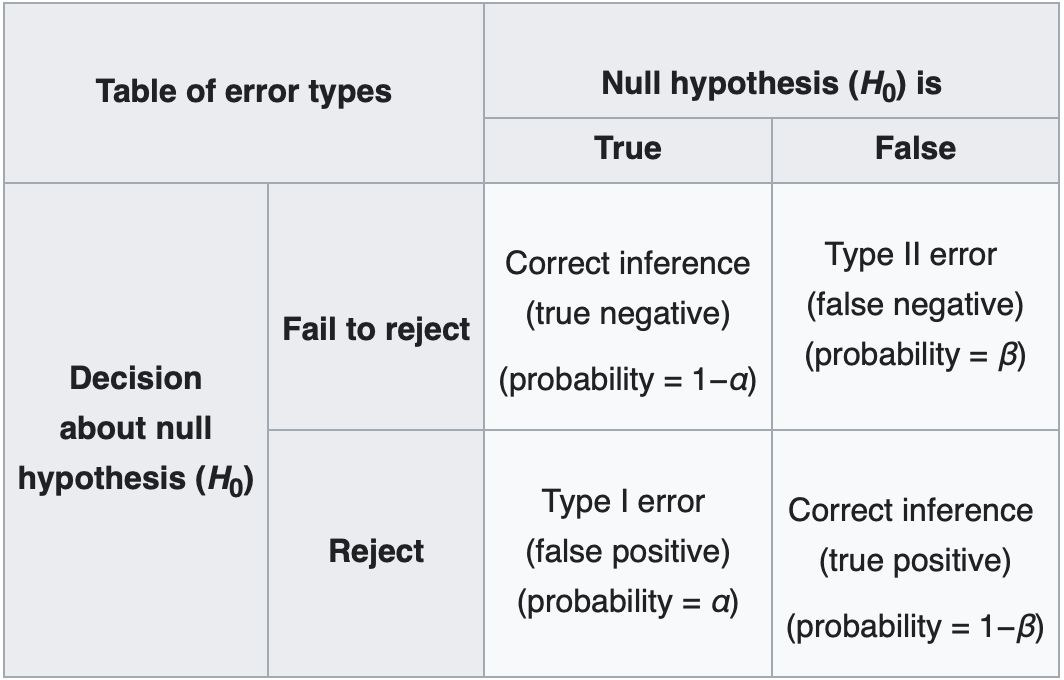
Before the test, we should decide on a probability of making a Type I error, $\alpha$, that we are comfortable with, called a “significance level”. Typical values are 5% and 1%, although if we’re claiming something crazy like a new particle, we better be very sure this isn’t a false positive; hence, we set a much lower significance level for these tests of $3\times10^{-7}$. (The significance of this value will be explained below.)

3.3. Deriving $p(\tilde{t}_s|s)$#

We can approximate $p(\tilde{t}_s|s)$ by generating several pseudo- or “toy” datasets assuming $s$ expected signal events. In this case, this means sampling possible values for $n, m$.

Note

One complication is that the $n, m$ distributions from which we want to sample (Eq. (3.1)) also depend on the nuisance parameter $b$. However, we’ll see that this won’t matter as much as we might expect.

num_toys = 10000
sbs = [
    [(5.0, 1.0), (5.0, 5.0), (5.0, 10.0)],
    [(100, 1), (100, 30), (100, 200)],
    [(10000, 100), (10000, 1000), (10000, 10000)],
]

fig, axs = plt.subplots(1, 3, figsize=(24, 6))
for i, sb in enumerate(sbs):
    for s, b in sb:
        # sample n, m according to our data model (Eq. 1)
        n, m = poisson.rvs(s + b, size=num_toys), poisson.rvs(b, size=num_toys)
        axs[i].hist(
            t_tilde_s(s, n, m),
            np.linspace(0, 6, 41),
            histtype="step",
            density=True,
            label=rf"$s = {int(s)}, b = {int(b)}$",
        )

    axs[i].legend()
    axs[i].set_xlabel(r"$\tilde{t}_s$")
    axs[i].set_ylabel(r"$p(\tilde{t}_s|s)$")

plt.show()

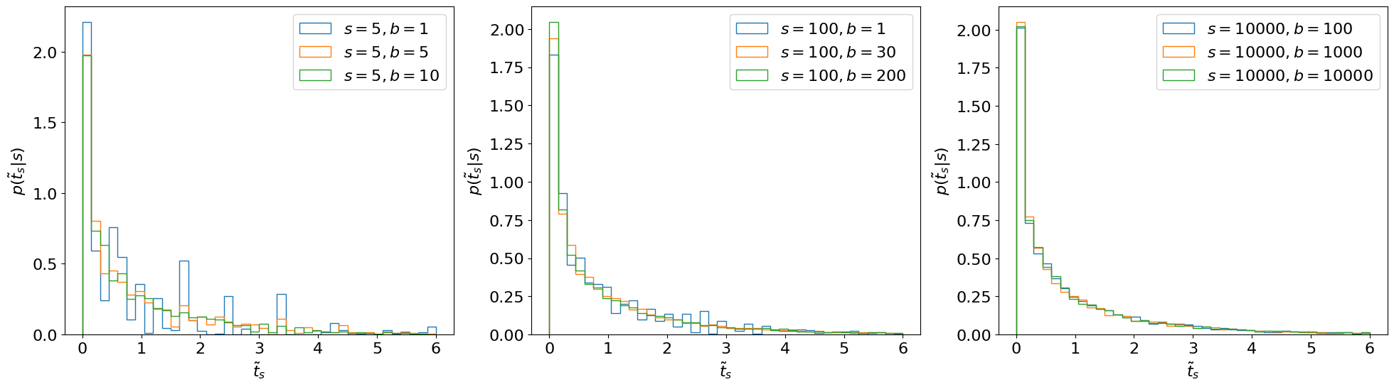
_images/f48ce870672006b97b8eeef74cf7f4ffaff41022f5b67407bca11beb3af62658.png — Fig. 3.1 Estimating $p(\tilde{t}_s|s)$ through toys.#

Observations

$p(\tilde{t}_s|s)$ does not depend on nuisance parameters ($b$) as long as $b$ is sufficiently large (this is a key reason for basing our test statistic on the profile likelihood).
In fact, $p(\tilde{t}_s|s)$ doesn’t even depend on $s$! (Again, as long as $s$ is large.)

Ref. [1] shows that, asymptotically, this distribution follows a $\chi^2$ distribution with degrees of freedom = # of parameters of interest. You can see the derivation in the reference therein but, essentially, like with most things in physics, this follows from Taylor expanding around the minimum…

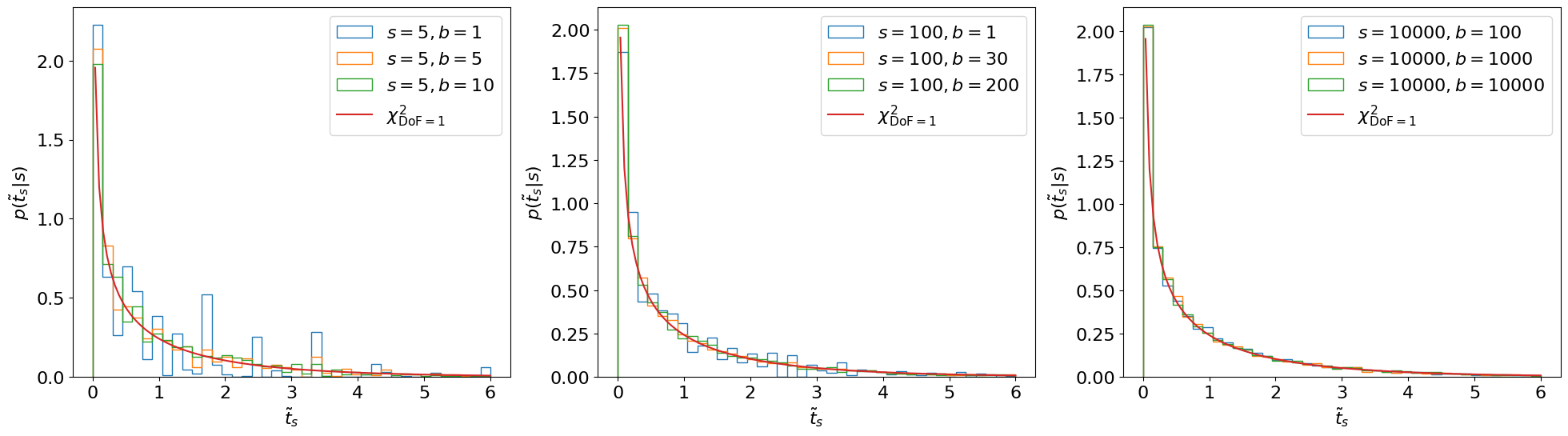
_images/5b34a87d4ad8e89414cc9411118da607f6a88a7a04a1bd93a08b9585b33f4fe8.png — Fig. 3.2 Asymptotic form of $p(\tilde{t}_s|s)$.#

This asymptotic form looks accurate even for $s, b$ as low as ~5.

Important

For cases where you can’t use the asymptotic form, Ref. [2] recommends using $b = \hat{\hat{b}}(s)$ when generating toys, so that you (approximately) maximise the agreement with the hypothesis.

3.4. $p$-values and Significance#

Now that we know the distribution of the test statistic $p(\tilde{t}_s|H_s) \equiv p(\tilde{t}_s|s)$, we can finally test $H_s$ with our experiment.

Let’s say we’re testing the hypothesis of $s = 10$ signal events in our model and we observe $n = 20, m = 5$ events. We can map this observation to our test statistic $\tilde{t}^\mathrm{obs}_s$:

s, n_obs, m_obs = 10, 20, 5
t_obs = t_tilde_s(s, n_obs, m_obs)
display(Latex(rf"$\tilde{{t}}^\mathrm{{obs}}_s = {t_obs:.2f}$"))

\[\tilde{t}^\mathrm{obs}_s = 1.07\]

And then see where this falls in our $p(\tilde{t}_s|s)$ distribution:

def get_toys(s, n_obs, m_obs, num_toys):
    """Generate toy data for a given s and observed n and m"""
    #  use b^^ for p(t_s|s) as recommended by Ref. 2
    b = bhathat(s, n_obs, m_obs)
    # sample n, m according to our data model (Eq. 1)
    n, m = poisson.rvs(s + b, size=num_toys), poisson.rvs(b, size=num_toys)

    return n, m


def get_p_ts(test_s, n_obs, m_obs, num_toys, toy_s=None):
    """
    Get the t_tilde_s test statistic distribution via toys.
    By default, the s we're testing is the same as the s we're using for toys,
    but this can be changed if necessary (as you will see later).
    """
    if toy_s is None:
        toy_s = test_s
    n, m = get_toys(toy_s, n_obs, m_obs, num_toys)
    return t_tilde_s(test_s, n, m)


def get_ps_val(test_s, n_obs, m_obs, num_toys, toy_s=None):
    """p value"""
    t_tilde_ss = get_p_ts(test_s, n_obs, m_obs, num_toys, toy_s)
    t_obs = t_tilde_s(test_s, n_obs, m_obs)
    p_val = np.mean(t_tilde_ss > t_obs)
    return p_val, t_tilde_ss, t_obs

s, n_obs, m_obs = 10, 20, 5
p_value_1, t_tilde_ss, t_obs = get_ps_val(s, n_obs, m_obs, num_toys)
p_value_1 = round(p_value_1, 1)

fig, ax = plt.subplots(figsize=(8, 6))
plot_p_ts(ax, s, n_obs, m_obs, t_tilde_ss, t_obs, p_value_1)
plt.show()

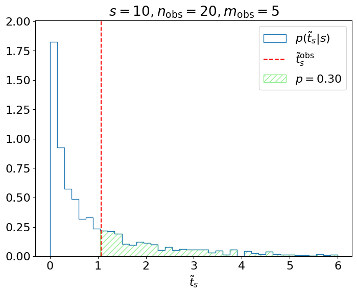
_images/bffade09e35180fb9344302771bedadad1d9afd08f51300fc7fa303bcbe14858.png — Fig. 3.3 Testing $H_s$.#

We care about, given $p(\tilde{t}_s|s)$, the probability of obtaining $\tilde{t}^\mathrm{obs}_s$ or a value more inconsistent with $H_s$; i.e., the green shaded region above. This is referred to as the $p$-value of the observation:

(3.3)#\[ p_s = \int_{\tilde{t}_\mathrm{obs}}^{\infty}p(\tilde{t}_s|s)\mathrm d \tilde{t}_s = 1 - F(\tilde{t}_\mathrm{obs}|s), \]

which is for this example, where

(3.4)#\[ F(\tilde{t}_s|s) = \int_{-\infty}^{\tilde{t}_s}p(\tilde{t}'_s|s)\mathrm d \tilde{t}'_s \]

is the cumulative distribution function (CDF) of $\tilde{t}_s$. We reject the hypothesis if this $p$-value is less than our chosen significance level $\alpha$; the idea being that if $H_s$ were true and we repeated this measurement many times, then the probability of a false-positive ($p$-value $\leq \alpha$) is exactly $\alpha$, as we intended.

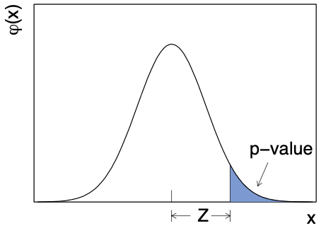
Often the $p$-value is also “converted” into a significance ($Z$), which is the corresponding number of standard deviations away from the mean in a Gaussian distribution

(3.5)#\[ Z = \Phi^{-1}(1-p), \]

where $\Phi$ is the CDF of the standard Gaussian. This is more easily illustrated in a figure (taken from Ref. [2]), where $\varphi$ is the standard Gaussian distribution:

_images/significance.png — Fig. 3.4 Significance from $p$-value, from Ref. [2].#

The significance for this example is, therefore:

# "ppf" = percent point function, which is what scipy calls the quantile function
Z_1 = round(norm.ppf(1 - p_value_1), 2)
display(Latex(f"$Z = {Z_1:.2f}$"))

\[Z = 0.52\]

We sometimes say that our measurement is (in)consistent or (in)compatible with $H$ at the $\sigma$ level, or within $1\sigma$, or … the list goes on.

3.5. Signal discovery#

Here, we were testing the signal hypothesis, but usually when we’re searching for a particle, we instead test the “background-only” hypothesis $H_0$ and decide whether or not to reject it. This means we want $\tilde{t}^\mathrm{obs}_0$ and $p(\tilde{t}_0|0)$ (below).

s, n_obs, m_obs = 0, 20, 5
p_value, t_tilde_ss, t_obs = get_ps_val(s, n_obs, m_obs, num_toys)
Z = norm.ppf(1 - p_value)

fig, ax = plt.subplots(figsize=(8, 6))
plot_p_ts(ax, s, n_obs, m_obs, t_tilde_ss, t_obs, p_value, Z, hlim=10)
plt.show()

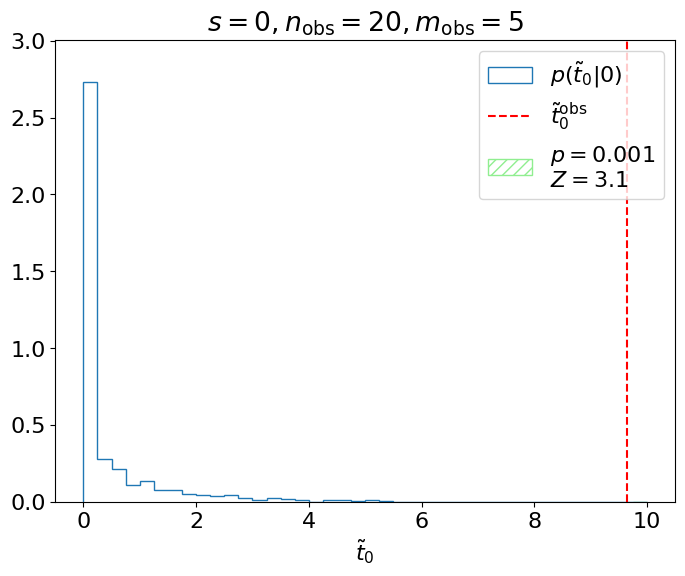
_images/5e90a33fa2fcdddda5867bf9e6232af8b3072a2dadf9a1083fdeba71e9962060.png — Fig. 3.5 Testing the background-only hypothesis.#

We could say for this experiment, therefore, that we exclude the background-only hypothesis at the “3 sigma” level. However, for an actual search for a new particle at the LHC, this is insufficient to claim a discovery, as the probability of a false positive at $3\sigma$, ~1/1000, is too high. The standard is instead set at $5\sigma$ for discovering new signals, corresponding to the $3\times10^{-7}$ significance level quoted earlier (we really don’t want to be making a mistake if we’re claiming to have discovered a new particle)! $3\sigma$, $4\sigma$, and $5\sigma$ are often referred to as evidence, observation, and discovery, respectively, of the signals we’re searching for.

3.6. Summary#

We went over the framework for hypothesis testing, which consists of:

Defining a test statistic $t$ to map data $\vec{x}$ (in our example, $\vec{x} = (n, m)$) to a single number.
Deriving the distribution of $t$ under the hypothesis being tested $p(t|H)$ by sampling from “toy” datasets assuming $H$.
Quantifying the compatibility of the observed data $\vec{x}_\mathrm{obs}$ with $H$ with the $p$-value or significance $Z$ of $t_\mathrm{obs}$ relative to $p(t|H)$.

This $p$-value / significance is what we then use to decide whether or not to exclude $H$. A particularly important special case of this is testing the background-only hypothesis when trying to discover a signal.

In Chapter 4, I’ll discuss going beyond testing to setting intervals and limits for parameters of interest.

Hypothesis Testing and Discovery Significance

Contents

3. Hypothesis Testing and Discovery Significance#

3.1. Recap#

3.2. Hypothesis testing#

3.3. Deriving \(p(\tilde{t}_s|s)\)#

3.4. \(p\)-values and Significance#

3.5. Signal discovery#

3.6. Summary#