Confidence Intervals and Limits

4. Confidence Intervals and Limits#

4.1. Recap#

We defined in Chapter 2 our probability model and likelihood function for a simple one bin counting experiment with $n$ events, $s$ signal and $b$ background, in our signal region and $m$ events, $b$ background, in our control region:

(4.1)#\[ P(n, m; s, b) = \frac{(s+b)^n e^{-(s+b)}}{n!} \cdot \frac{b^m e^{-b}}{m!} = L(s, b), \]

and our test statistic $\tilde{t}_s$:

(4.2)#\[\begin{split} \tilde{\lambda}(s) = \left\{ \begin{array}{ll} \frac{L(s, \hat{\hat{b}}(s))}{L(\hat{s}, \hat{b})}, & \mbox{$\hat{s}\geq0$}.\\ \frac{L(s, \hat{\hat{b}}(s))}{L(0, \hat{\hat{b}}(0))}, & \mbox{$\hat{s}<0$}. \end{array} \right., \quad \tilde{t}_s=-2\ln \tilde{\lambda}(s), \end{split}\]

and solved for $\hat{s}, \hat{b}, \hat{\hat{b}}(s)$ for given $n, m$ to find an analytic form for $t_s$.

In Chapter 3, we translated this to a probability distribution of $\tilde{t}_s$ under a particular signal hypothesis $H_s$, and quantified the compatibility of our observation based on the $p$-value $p_s$ of the observed test statistic $\tilde{t}_s^\mathrm{obs}$:

(4.3)#\[ p_s = \int_{\tilde{t}_\mathrm{obs}}^{\infty}p(\tilde{t}_s|s)\mathrm d \tilde{t}_s, \]

and it’s associated significance.

Code from previous parts:

4.2. Confidence intervals using the Neyman construction#

The machinery from Part 2 can be extended straightforwardly to extracting “confidence intervals” for our parameters of interest (POIs): a range of values of the POIs that are allowed, based on the experiment, at a certain “confidence level” (CL), e.g. 68% or 95%. Very similar to the idea of the significance level, the CL is defined such that if we were to repeat the experiment many times, a 95%-confidence-interval must contain, or cover, the true value of the parameter 95% of the time.

We can ensure this for any given CL by solving Eq. (4.3) for a $p$-value of $1 - \mathrm{CL}$:

(4.4)#\[ p = 1 - \mathrm{CL} = \int_{\tilde{t}^\mathrm{obs}_s}^{\infty}p(\tilde{t}_s|s_\pm)\mathrm d \tilde{t}_s, \]

where $s_-$ and $s_+$ are the lower and upper limits on $s$, respectively.

We solve this by scanning $s$ and finding the values of $s$ for which the RHS $= 1 - \mathrm{CL}$. Continuing with our above example:

def get_limits(s_scan: list, n_obs: int, m_obs: int, num_toys: int, CL: float = 0.95):
    t_tilde_scan = []  # saving sampled test statistics for each s
    t_obs_scan = []  # saving t_obs for each s
    p_val_scan = []  # saving p-value for each s

    for s in s_scan:
        p_val, t_tilde_ss, t_obs = get_ps_val(s, n_obs, m_obs, num_toys)
        t_obs_scan.append(t_obs)
        t_tilde_scan.append(t_tilde_ss)
        p_val_scan.append(p_val)

    # find the values of s that give p_value ~= 1 - CL
    pv_cl_diff = np.abs(np.array(p_val_scan) - (1 - CL))
    # split into lower and upper half to get lower and upper limits
    # (not the best way to do this, but works for now...)
    half_num_s = int(len(s_scan) / 2)
    s_low = s_scan[np.argsort(pv_cl_diff[:half_num_s])[0]]
    s_high = s_scan[half_num_s:][np.argsort(pv_cl_diff[half_num_s:])[0]]

    return s_low, s_high, t_tilde_scan, t_obs_scan, p_val_scan

num_toys = 10000
n_obs, m_obs = 20, 5
s_scan = np.arange(0, 30.1, 0.05)  # scanning s over these values
s_low, s_high, t_tilde_scan, t_obs_scan, p_val_scan = get_limits(s_scan, n_obs, m_obs, num_toys)
s_low, s_high = round(s_low, 1), round(s_high, 1)
display(Latex(f"$s \in [{s_low:.1f}, {s_high:.1f}]$"))

\[s \in [6.0, 25.6]\]

_images/c93cbb9fede682d41fdfc59d883bf8f9ecdd79c2716b57a56bd6cf69cb764d3a.png — Fig. 4.1 Demonstration of the Neyman construction for a 95% confidence interval. Left: Scanning $p(\tilde{t}_s|s)$ using 10,000 toys each for different values of $s$. Right: Contour plot of the $p$-values for different $\tilde{t}_s$’s as a function of $s$, with the observed $t^\mathrm{obs}_s$ in red. The points at which $t^\mathrm{obs}_s$ intersects with the $p$-value = 0.05 contour are marked in black and signify the limits of the 95% confidence interval for $s$ - in this case, $[$, $]$.#

This procedure of inverting the hypothesis test by scanning along the values of the POIs is called the “Neyman construction”.

Tip

One subtlety to remember is that, in principle, we should also be scanning over the nuisance parameters ($b$) when estimating the $p$-values. However, this would be very computationally expensive so in practice we continue to use $b = \hat{\hat{b}}(s)$, to always (approximately) maximise the agreement with the hypothesis. Ref. [2] calls this trick “profile construction”.

4.3. Upper Limits#

Typically if a search does not have enough sensitivity to directly observe a new signal, we instead quote an upper limit on the signal strength. This is similar in practice to the Neyman construction for confidence intervals, solving Eq. (4.4) only for the upper boundary. However, an important difference is that when setting upper limits, we have to modify the test statistic so that a best-fit signal strength greater than the expected signal ($\hat{s} > s$) does not lower the compatibility with $H_s$:

(4.5)#\[\begin{split} \tilde{q}(s) = \left\{ \begin{array}{ll} \tilde{t}(s), & \mbox{$\hat{s} < s$}.\\ 0, & \mbox{$\hat{s} \geq s$}. \end{array} \right. = \left\{ \begin{array}{ll} -2\ln\tilde{\lambda}(s), & \mbox{$\hat{s} < s$}.\\ 0, & \mbox{$\hat{s} \geq s$}. \end{array} \right. = \left\{ \begin{array}{ll} -2\ln\frac{L(s, \hat{\hat{b}}(s))}{L(0, \hat{\hat{b}}(0))}, & \mbox{$\hat{s}<0$}.\\ -2\ln\frac{L(s, \hat{\hat{b}}(s))}{L(\hat{s}, \hat{b})}, & \mbox{0 $\leq \hat{s} < s$}.\\ 0, & \mbox{$\hat{s} \geq s$}. \end{array} \right. \end{split}\]

The upper limit test statistic $\tilde{q}(s)$ is set to 0 for $\hat{s} > s$ so that this situation does not contribute to the $p$-value integral in Eq. (4.3). This is what this looks like:

def q_tilde_s(s, n, m):
    ts = np.array(t_s(s, n, m))

    neg_shat_mask = shat(n, m) < 0  # find when s^ is < 0
    t_zero = t_zero_s(s, n, m)
    # replace values where s^ < 0 with lam_zero
    ts[neg_shat_mask] = t_zero[neg_shat_mask]

    upper_shat_mask = shat(n, m) > s
    ts[upper_shat_mask] = 0

    return ts.squeeze()

nms = [(10.0, 4.0), (12.0, 10.0), (60, 50.0)]  # sample (n, m) observations

fig, ax = plt.subplots(figsize=(12, 8))
plot_ts_qs(ax, nms)
plt.show()

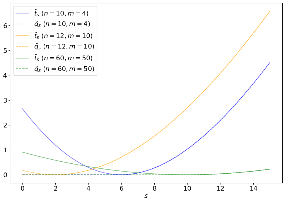
_images/0ca98a9cc221ea852739e8b931e87ac8d4b2cf73292387f0f5121bf9e2b740fc.png — Fig. 4.2 Comparing $\tilde{t}_s$ and $\tilde{q}_s$.#

Note

As you may expect from the plot above, the distribution $p(\tilde{q}_s|s)$ no longer behaves like a standard $\chi^2$ but, instead, as a “half-$\chi^2$”. This is essentially a $\chi^2$ + a delta function at 0 (since, under the signal hypothesis, on average there will be an over-fluctuation half the time, for which $\tilde{q}_s = 0$), as shown below.

sbs = [(10, 50), (100, 80), (20, 160)]  # sample s, b
fig, axs = plt.subplots(1, 3, figsize=(24, 6))
plot_p_ts_qs(axs, sbs)
plt.show()

_images/b2c8b3ece0d83d814f3e3210e7d985c10c5636593e060f93fa920d9db5b99a2d.png — Fig. 4.3 Comparing $p(\tilde{t}_s|s)$ and $p(\tilde{q}_s|s)$.#

And this is what our example above looks like, solving for an upper limit on $s$ rather than a confidence interval:

def get_p_qs(test_s, n_obs, m_obs, num_toys, toy_s=None):
    """
    Get the q_tilde_s test statistic distribution via toys.
    By default, the s we're testing is the same as the s we're using for toys,
    but this can be changed if necessary (as you will see later).
    """
    if toy_s is None:
        toy_s = test_s
    n, m = get_toys(toy_s, n_obs, m_obs, num_toys)
    return q_tilde_s(test_s, n, m)


def get_pval_qs(test_s, n_obs, m_obs, num_toys, toy_s=None):
    """p value"""
    q_tilde_ss = get_p_qs(test_s, n_obs, m_obs, num_toys, toy_s)
    q_obs = q_tilde_s(test_s, n_obs, m_obs)
    p_val = np.mean(q_tilde_ss > q_obs)
    return p_val, q_tilde_ss, q_obs


def get_upper_limit(s_scan: list, n_obs: int, m_obs: int, num_toys: int, CL: float = 0.95):
    q_tilde_scan = []  # saving sampled test statistics for each s
    q_obs_scan = []  # saving q_obs for each s
    p_val_scan = []  # saving p-value for each s

    for s in s_scan:
        p_val, q_tilde_ss, q_obs = get_pval_qs(s, n_obs, m_obs, num_toys)
        q_obs_scan.append(q_obs)
        q_tilde_scan.append(q_tilde_ss)
        p_val_scan.append(p_val)

    # find the values of s that give p_value ~= 1 - CL
    pv_cl_diff = np.abs(np.array(p_val_scan) - (1 - CL))
    s_upper = s_scan[np.argsort(pv_cl_diff)[0]]

    return s_upper, q_tilde_scan, q_obs_scan, p_val_scan

n_obs, m_obs = 20, 5
s_scan = np.arange(0, 30.1, 0.05)  # scanning s over these values
s_upper_qs, q_tilde_scan, q_obs_scan, p_val_scan = get_upper_limit(s_scan, n_obs, m_obs, num_toys)
s_upper_qs = round(s_upper_qs, 1)
display(Latex(f"$s \leq {s_upper_qs:.1f}$"))

\[s \leq 24.0\]

fig, axs = plt.subplots(1, 2, figsize=(22, 8))
# plot p(t_s|s) for all values of s
plot_2d_p_ts_s(fig, axs[0], t_tilde_s, s_scan, ts="q")
# plot the p-values as a function of t_s and s
plot_pval_levels(axs[1], s_scan, q_tilde_scan, q_obs_scan, s_upper_qs, ts="q")
plt.show()

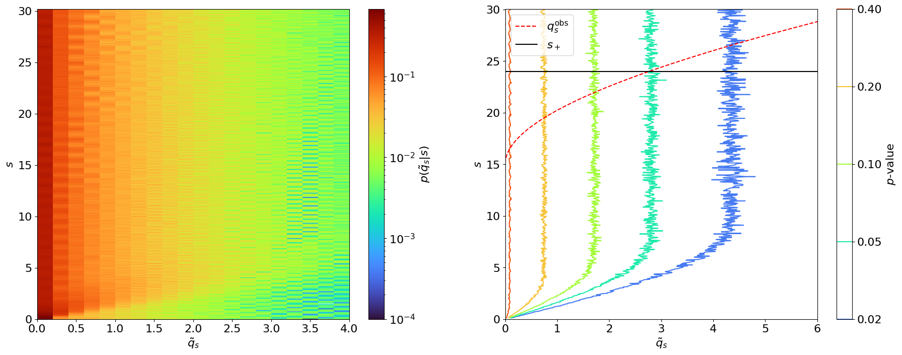
_images/991432bc8d165ed521cf0c0136da0c0c570ba1cb582ee742ef96cc08945c6fee.png — Fig. 4.4 Extending the Neyman construction to an upper limit on $s$. Left: Scanning $p(\tilde{q}_s|s)$ using 10,000 toys each for different values of $s$. Right: Contour plot of the $p$-values for different $\tilde{q}_s$’s as a function of $s$, with the observed $q^\mathrm{obs}_s$ in red. The point at which $q^\mathrm{obs}_s$ intersects with the $p$-value = 0.05 contour is marked in black and signifies the upper limit at 95% CL.#

$p(\tilde{q}_s|s)$ is shifted to the left with respect to $p(\tilde{t}_s|s)$; hence, the upper limit of is slightly lower than the upper bound of the 95% confidence interval we derived using $\tilde{t}_s$.

4.4. The CL$_s$ criterion#

I now introduce two conventions related to hypothesis testing and searches in particle physics. Firstly (the simple one), the POI $s$ is usually re-parametrized as:

(4.6)#\[ s \rightarrow \mu \cdot s, \]

where now $\mu$ is the POI, referred to as the “signal strength”, and $s$ is a fixed value representing the number of signal events we expect to see for the nominal signal strength $\mu$ of 1. For the example above, if we expect $s = 10$ signal events, then we would quote the upper limit as $ / s =$ 2.4 on $\mu$ at 95% CL.

The second, important, convention is that we use a slightly different criterion for our confidence intervals, called “CL$_s$”. This is motivated by situations where we have little sensitivity to the signal we’re searching for. For example, let’s say we expect $s = 10$ and observe $n = 70, m = 100$. Really, what this should indicate is that our search is not at all sensitive, since our search region is completely dominated by background and, hence, we should not draw strong conclusions about the signal strength. However, let’s see what limit the above procedure sets fo this experiment:

s, n_obs, m_obs = 10, 70, 100
s_scan = np.arange(0, 10, 0.01)  # scanning s over these values
s_upper, q_tilde_scan, q_obs_scan, p_val_scan = get_upper_limit(s_scan, n_obs, m_obs, num_toys)
display(Latex(f"$\mu \leq {s_upper / s:.3f}$"))

\[\mu \leq 0.024\]

We end up setting an aggressive limit on $\mu$ and excluding $\mu = 1$ (at 95% CL). This is undesirable given the complete lack of sensitivity to the signal.

The CL$_s$ method solves this problem by considering both the $p$-value of the signal + background hypothesis $H_s$ (referred to as $p_{s+b}$ or just $p_\mu$ for short), and the $p$-value of the background-only hypothesis $H_0$ ($p_b$), to define a new criterion:

(4.7)#\[ p_\mu' = \cfrac{p_\mu}{1 - p_b} \]

In cases where the signal region is completely background dominated, the compatibility with the background-only hypothesis should be high, so $p_b \sim 1$ and, hence, $p_\mu'$ will be increased (as we want). On the other hand, for more sensitive regions, compatibility should be lower $\Rightarrow p_b \sim 0$ and $p_\mu' \sim p_\mu$.

To be explicit, here

(4.8)#\[ p_b = \int^{\tilde{t}_\mathrm{obs}}_{-\infty}p(\tilde{t}_s|0)\mathrm d \tilde{t}_s, \]

where we should note that:

Note

We’re looking at the distribution of $\tilde{t}_s$, not $\tilde{t}_0$, under the background-only hypothesis, since the underlying test is of $H_s$, not $H_0$; and
We’re integrating up to $\tilde{t}_\mathrm{obs}$, unlike for $p_s$, because lower $\tilde{t}$ means greater compatibility with the background-only hypothesis.

Let’s see what this looks like:

fig, axs = plt.subplots(1, 2, figsize=(22, 8))

s, n_obs, m_obs = 10, 20, 5
p_mu, t_tilde_ss, t_obs = get_ps_val(s, n_obs, m_obs, num_toys)
p_b, t_tilde_sb, t_obs_b = get_ps_val(s, n_obs, m_obs, num_toys, toy_s=0)
p_b = 1 - p_b  # invert integral for background-only p_value
plot_pmu_pb(axs[0], s, n_obs, m_obs, t_tilde_ss, t_tilde_sb, t_obs, p_mu, p_b, hlim=14)

s, n_obs, m_obs = 10, 70, 100
p_mu, t_tilde_ss, t_obs = get_ps_val(s, n_obs, m_obs, num_toys)
p_b, t_tilde_sb, t_obs_b = get_ps_val(s, n_obs, m_obs, num_toys, toy_s=0)
p_b = 1 - p_b
plot_pmu_pb(axs[1], s, n_obs, m_obs, t_tilde_ss, t_tilde_sb, t_obs, p_mu, p_b)

plt.show()

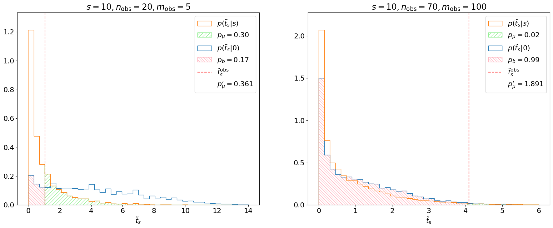
_images/3b5e7dcc835d336f42d99e8a730cc62a86d867815ff09739fb5bb2aeb6bbc8fc.png — Fig. 4.5 Demonstration of CL$_s$ criterion.#

We see that for our first example (left), the background-only distribution is shifted to the right of the $s+b$ distribution. This indicates that the experiment is sensitive to $\mu$ and indeed $p_\mu' \sim p_\mu$. In the second example, however, the search is not sensitive and, hence, the background-only and $s+b$ distributions almost completely overlap, meaning $p_b \sim 1$ and $p_\mu' >> p_\mu$.

Note

Unlike $p(\tilde{t}_s|s)$, $p(\tilde{t}_s|0)$ doesn’t follow a simple $\chi^2$; asymptotically, it is closer to a noncentral $\chi^2$, as discussed in Ref. [1], which we’ll get to in Parts 5-6.

Finally, let’s see if our upper limit make more sense using CL$_s$:

def get_limits_CLs(s_scan: list, n_obs: int, m_obs: int, num_toys: int, CL: float = 0.95):
    p_cls_scan = []  # saving p-value for each s

    for s in s_scan:
        p_mu, t_tilde_sb, t_obs = get_ps_val(s, n_obs, m_obs, num_toys)
        p_b, t_tilde_sb, t_obs = get_ps_val(s, n_obs, m_obs, num_toys, toy_s=0)
        p_b = 1 - p_b
        p_cls_scan.append(p_mu / (1 - p_b))

    # find the values of s that give p_value ~= 1 - CL
    pv_cl_diff = np.abs(np.array(p_cls_scan) - (1 - CL))
    half_num_s = int(len(s_scan) / 2)
    s_low = s_scan[np.argsort(pv_cl_diff[:half_num_s])[0]]
    s_high = s_scan[half_num_s:][np.argsort(pv_cl_diff[half_num_s:])[0]]

    return s_low, s_high


def get_upper_limit_CLs(s_scan: list, n_obs: int, m_obs: int, num_toys: int, CL: float = 0.95):
    p_cls_scan = []  # saving p-value for each s

    for s in s_scan:
        p_mu, q_tilde_sb, q_obs = get_pval_qs(s, n_obs, m_obs, num_toys)
        p_b, q_tilde_sb, q_obs = get_pval_qs(s, n_obs, m_obs, num_toys, toy_s=0)
        p_b = 1 - p_b
        p_cls_scan.append(p_mu / (1 - p_b))

    # find the values of s that give p_value ~= 1 - CL
    pv_cl_diff = np.abs(np.array(p_cls_scan) - (1 - CL))
    s_upper = s_scan[np.argsort(pv_cl_diff)[0]]

    return s_upper

s, n_obs, m_obs = 10, 70, 100
s_scan = np.arange(0, 30, 0.1)  # scanning s over these values
s_upper = get_upper_limit_CLs(s_scan, n_obs, m_obs, num_toys)
display(Latex(f"$\mu \leq {s_upper / s:.1f}$"))

\[\mu \leq 1.5\]

Indeed, we see a looser, more conservative, upper limit. We can also confirm that the limit for our first example, which had better sensitivity, stays the same:

n_obs, m_obs = 20, 5
s_scan = np.arange(0, 30.1, 0.05)  # scanning s over these values
s_upper = get_upper_limit_CLs(s_scan, n_obs, m_obs, num_toys)
display(Latex(f"$\mu \leq {s_upper / s:.1f}$"))

\[\mu \leq 2.4\]

4.5. Summary#

We extended the framework for hypothesis testing to derive frequentist confidence intervals for parameters of interest by solving for particular $p$-values, called the “Neyman construction”. For upper limits, we find that we need to use a further modified test statistic $\tilde{q}_\mu$ and the “CL$_s$” criterion to avoid excluding signals for which we don’t have sensitivity. In Chapter 5, I’ll discuss the concepts of expected significances and limits, which are important to estimate our experiment’s sensitivity before collecting or looking at the data.

Confidence Intervals and Limits

Contents

4. Confidence Intervals and Limits#

4.1. Recap#

4.2. Confidence intervals using the Neyman construction#

4.3. Upper Limits#

4.4. The CL\(_s\) criterion#

4.5. Summary#