Asymptotic Form of the MLE

6. Asymptotic Form of the MLE#

6.1. Recap#

We have been working with a probability model and likelihood function for a simple one bin counting experiment with \(n\) observed, \(s\) expected signal, and \(b\) expected background events in our signal region and \(m\) observed and \(b\) expected background events, in our control region, with the signal strength parametrized by \(\mu\):

(6.1)#\[ P(n, m; \mu s, b) = \frac{(\mu s+b)^n e^{-(\mu s+b)}}{n!} \cdot \frac{b^m e^{-b}}{m!} = L( \mu, b), \]

The negative-log-likelihood (NLL) is:

(6.2)#\[-\ln L = \ln n! + \ln m! + \mu s + 2b - n\ln(\mu s+b) - m \ln b\]

Code from previous parts:

Show code cell source Hide code cell source

def get_toys_sb(s, b, num_toys):
    """Generate toy data for a given s and b"""
    # sample n, m according to our data model (Eq. 1)
    n, m = poisson.rvs(s + b, size=num_toys), poisson.rvs(b, size=num_toys)
    return n, m


def get_toys(s, n_obs, m_obs, num_toys):
    """Generate toy data for a given s and observed n and m"""
    #  use b^^ for p(t_s|s) as recommended by Ref. 2
    b = bhathat(s, n_obs, m_obs)
    return get_toys_sb(s, b, num_toys)


def get_p_ts(test_s, n_obs, m_obs, num_toys, toy_s=None):
    """
    Get the t_tilde_s test statistic distribution via toys.
    By default, the s we're testing is the same as the s we're using for toys,
    but this can be changed if necessary (as you will see later).
    """
    if toy_s is None:
        toy_s = test_s
    n, m = get_toys(toy_s, n_obs, m_obs, num_toys)
    return t_tilde_s(test_s, n, m)


def get_ps_val(test_s, n_obs, m_obs, num_toys, toy_s=None):
    """p value"""
    t_tilde_ss = get_p_ts(test_s, n_obs, m_obs, num_toys, toy_s)
    t_obs = t_tilde_s(test_s, n_obs, m_obs)
    p_val = np.mean(t_tilde_ss > t_obs)
    return p_val, t_tilde_ss, t_obs


def get_p_qs(test_s, n_obs, m_obs, num_toys, toy_s=None):
    """
    Get the q_tilde_s test statistic distribution via toys.
    By default, the s we're testing is the same as the s we're using for toys,
    but this can be changed if necessary (as you will see later).
    """
    if toy_s is None:
        toy_s = test_s
    n, m = get_toys(toy_s, n_obs, m_obs, num_toys)
    return q_tilde_s(test_s, n, m)


def get_pval_qs(test_s, n_obs, m_obs, num_toys, toy_s=None):
    """p value"""
    q_tilde_ss = get_p_qs(test_s, n_obs, m_obs, num_toys, toy_s)
    q_obs = q_tilde_s(test_s, n_obs, m_obs)
    p_val = np.mean(q_tilde_ss > q_obs)
    return p_val, q_tilde_ss, q_obs


def get_limits_CLs(s_scan: list, n_obs: int, m_obs: int, num_toys: int, CL: float = 0.95):
    p_cls_scan = []  # saving p-value for each s

    for s in s_scan:
        p_mu, t_tilde_sb, t_obs = get_ps_val(s, n_obs, m_obs, num_toys)
        p_b, t_tilde_sb, t_obs = get_ps_val(s, n_obs, m_obs, num_toys, toy_s=0)
        p_b = 1 - p_b
        p_cls_scan.append(p_mu / (1 - p_b))

    # find the values of s that give p_value ~= 1 - CL
    pv_cl_diff = np.abs(np.array(p_cls_scan) - (1 - CL))
    half_num_s = int(len(s_scan) / 2)
    s_low = s_scan[np.argsort(pv_cl_diff[:half_num_s])[0]]
    s_high = s_scan[half_num_s:][np.argsort(pv_cl_diff[half_num_s:])[0]]

    return s_low, s_high


def get_upper_limit_CLs(s_scan: list, n_obs: int, m_obs: int, num_toys: int, CL: float = 0.95):
    p_cls_scan = []  # saving p-value for each s

    for s in s_scan:
        p_mu, q_tilde_sb, q_obs = get_pval_qs(s, n_obs, m_obs, num_toys)
        p_b, q_tilde_sb, q_obs = get_pval_qs(s, n_obs, m_obs, num_toys, toy_s=0)
        p_b = 1 - p_b
        p_cls_scan.append(p_mu / (1 - p_b))

    # find the values of s that give p_value ~= 1 - CL
    pv_cl_diff = np.abs(np.array(p_cls_scan) - (1 - CL))
    s_upper = s_scan[np.argsort(pv_cl_diff)[0]]

    return s_upper

6.2. Introduction#

So far, we have discussed how to extract meaningful statistical results from HEP experiments by making extensive use of pseudodata / toy experiments to estimate the sampling distributions of profile-likelihood-ratio-based test statistics. While this worked nicely for our simple counting experiment, generating a sufficiently large number of toys can quickly become computationally intractable for the more complex searches (and statistical combinations of searches) that are increasingly prevalent at the LHC, containing at times up to thousands of bins and nuisance parameters. This and the following section discuss a way to approximate these sampling distributions without the need for pseudodata. This was introduced in the famous “CCGV” paper [1] in 2011, and has since become the de-facto procedure at the LHC.

As previously discussed, the distributions \(p(\tilde{t}_\mu|\mu')\) and \(p(\tilde{q}_\mu|\mu')\) (where, in general, \(\mu' \neq \mu\)) have similar forms regardless of the nuisance parameters (or sometimes even the POIs). This is not a coincidence: we will now derive their “asymptotic”, i.e. in the large sample limit, forms, starting first with asymptotic form of the maximum likelihood estimator (MLE).

It is important to remember that the MLE \(\hat \mu\) of \(\mu\) is a random variable with its own probability distribution. We can estimate it as always by sampling toys:

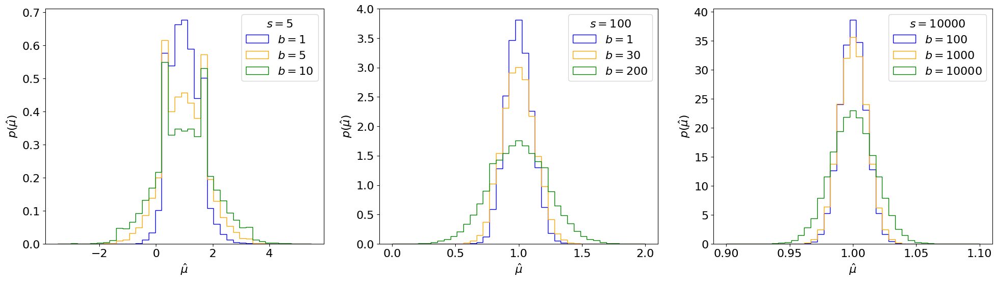
_images/cf042bf1b957841a345454794a4cc2653139c6f408607410c619cb3000baefe3.png — Fig. 6.1 Distribution of the MLE of \(\mu\) for different \(s\) and \(b\) produced using 30,000 toy experiments each. (Note the x-axis range is becoming narrower from the left-most to the right-most plot.)#

You may notice that \(p(\hat \mu)\) follows a Gaussian as the number of events \(N\) increases:

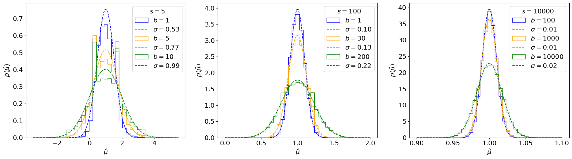
_images/74561178a5b358be5c0c13c7774d1102fd0fb65564b5e5eaeaa4877e319a4ae2.png — Fig. 6.2 Gaussian fits to distributions from Fig. 5.1 of the MLE of \(\mu\) for different \(s\) and \(b\).#

We will now show this to be true generally. You are welcome to skip ahead to the result if you’re not interested in the derivation.

6.3. Background statistics#

First, we need some statistics concepts and results:

Lightning Statistics

Let the log-likelihood \(\ln L(\mu) \equiv l(\mu)\).

The derivative of the NLL \(-l'(\mu)\) is called the score \(s(\mu)\). It has a number of useful properties:

Its expectation value at \(\mu'\): \(\mathbb E_{\mu = \mu'}[s(\mu')] = 0\).
Its variance \(\mathrm {Var} [s(\mu)] = - \mathbb E [l''(\mu)]\).

\(- \mathbb E [l''(\mu)] \equiv \mathcal I(\mu)\) is called the Fisher information. It quantifies the information our data contains about \(\mu\) and importantly, as we’ll see, it (approximately) represents the inverse of the variance of \(\hat \mu\). More generally, for multiple parameters, \(\mathcal I_{ij}(\mu) = - \mathbb E [\frac{\partial^2 l}{\partial \mu_i \partial \mu_j}]\) is the Fisher information matrix. It is also commonly called the covariance matrix.

Putting this together, by the central limit theorem, this means \(p(s(\mu'))\) follows a normal distribution with mean 0 and variance \(\mathcal I(\mu')\), up to terms of order \(\mathcal O(\frac{1}{\sqrt{N}})\):

(6.3)#\[ s(\mu') \xrightarrow{\sqrt{N} >> 1} \mathcal N(0, \sqrt{\mathcal I(\mu')}), \]

where \(N\) represents the data sample size.

6.3.1. Fisher Information#

For our simple counting experiment, the Fisher information matrix \(\mathcal I(\mu, b)\) can be found by taking second derivatives of Eq. (6.2). The \(\mathcal I_{\mu\mu}\) term, for example, is:

(6.4)#\[ \mathcal I_{\mu\mu}(\mu, b) = - \mathbb E[\partial^\mu\partial^\mu l(\mu, b)] = \mathbb E \bigg[n \cdot \cfrac{s^2}{(\mu s + b)^2}\bigg] = \mathbb E[n] \cdot \cfrac{s^2}{(\mu s + b)^2} = \cfrac{(\mu' s + b') s^2}{(\mu s + b)^2}. \]

In the last step we use the fact that \(\mathbb E[n]\) under true \(\mu = \mu', b = b'\), is \(\mu' s + b'\). For the remainder of this section, \(\mathcal I(\mu, b)\) will always be evaluated at the true values of the parameters (the reason for this is discussed below), so this can be simplified to \(\mathcal I_{\mu\mu}(\mu', b') = \frac{s^2}{\mu' s + b'}\).

This is what it looks like:

def get_fisher_mu_mu(mu, s, b):
    # assuming here that mu and b equal their true values
    return (s**2) / (mu * s + b)

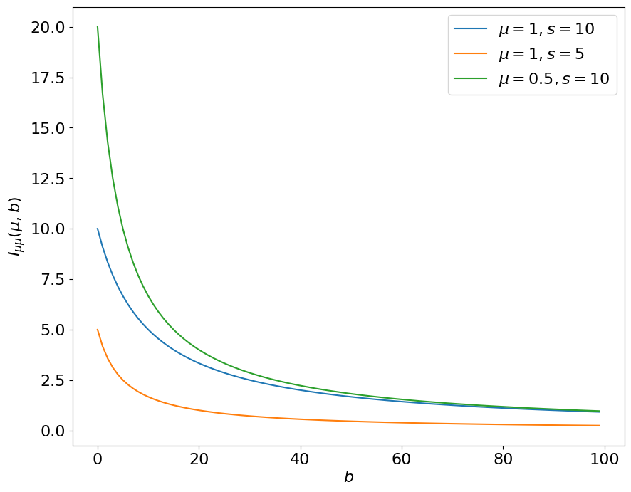
_images/a5512fa2580a50a88f8aba6518c3521c18bcee3760916831a67b28a35949c961.png — Fig. 6.3 The Fisher information \(\mathcal I_{\mu\mu}(\mu, b)\) for different \(\mu\) and \(s\), as a function of the expected background \(b\).#

The Fisher information captures the fact that as \(b\) increases, we lose sensitivity to - or information about - \(\mu\). Exercise 🙃: why are the orange and green values different?

For completeness (and since we’ll need it below) the full Fisher information matrix for our problem, repeating the steps in Eq. (6.4), is:

(6.5)#\[\begin{split} \mathcal I(\mu', b') = \begin{pmatrix}\mathcal I_{\mu\mu} & \mathcal I_{\mu b} \\ \mathcal I_{b\mu} & \mathcal I_{bb}\end{pmatrix}(\mu', b') = \begin{pmatrix} \frac{s^2}{\mu' s + b'} & \frac{s}{\mu' s + b'} \\ \frac{s}{\mu' s + b'} & \frac{1}{\mu' s + b'} + \frac{1}{b'} \end{pmatrix} \end{split}\]

6.4. Derivation#

We now have enough background to derive the asymptotic form of the MLE. We do this for the 1D case by Taylor-expanding the score of \(\hat \mu\), \(l'(\hat\mu)\) - which we know to be \( = 0\) - around \(\mu'\):

(6.6)#\[\begin{split} l'(\hat\mu) = l'(\mu') + l''(\mu')(\hat\mu - \mu') + \mathcal O((\hat\mu - \mu')^2) = 0 \\ \Rightarrow \hat\mu - \mu' \simeq - \cfrac{l'(\mu')}{l''(\mu')} \xrightarrow{\sqrt{N} >> 1} \cfrac{1}{\mathcal I(\mu')}N(0, \sqrt{\mathcal I(\mu')}) = N\bigg(0, \frac{1}{\sqrt{\mathcal I(\mu')}}\bigg), \end{split}\]

where we plugged in the distribution of \(l'(\mu')\) from Eq. (6.3), claimed \(l''(\mu')\) asymptotically equals its expectation value \(\mathbb E[l''(\mu')] = \mathcal I(\mu')\) by the law of large numbers, and are ignoring the \(\mathcal O((\hat\mu - \mu')^2)\) term.

For multiple parameters, \(\mathcal I\) is a matrix so the variance is its matrix inverse:

(6.7)#\[ \hat\mu - \mu' \simeq N(0, \sqrt{\mathcal I^{-1}_{\mu\mu}(\mu', b')}), \]

6.5. Result#

Thus, we see that \(\hat \mu\) asymptotically follows a normal distribution around the true \(\mu\) value, \(\mu'\), with a variance \(\sigma_{\hat\mu}^2 = \mathcal I^{-1}_{\mu\mu}(\mu', b')\), up to \(\mathcal O (1/\sqrt{N})\) terms. Intuitively, from the definition of the Fisher information \(\mathcal I\), we can interpret this as saying that the more information we have about \(\mu\) from the data, the lower the variance should be on \(\hat \mu\).

For our counting experiment, inverting \(\mathcal I\) from Eq. (6.5) gives us

(6.8)#\[ \sigma_{\hat\mu} = \sqrt{\mathcal I^{-1}_{\mu\mu}(\mu', b')} = \cfrac{\sqrt{\mu' s + 2b'}}{s}. \]

Note

Note that, as we might expect, this scales as \(\sim \sqrt{b}\), which is the uncertainty of our Poisson nuisance parameter \(b\) - showing mathematically why we want to keep uncertainties on nuisance parameters as low as possible.

Let’s see how closely this matches the toy-based distributions from earlier, this time varying the true signal strength \(\mu'\) as well:

def get_asym_std(mu, s, b):
    """Inputs should be the "true" mu and b values"""
    return np.sqrt(mu * s + 2 * b) / s

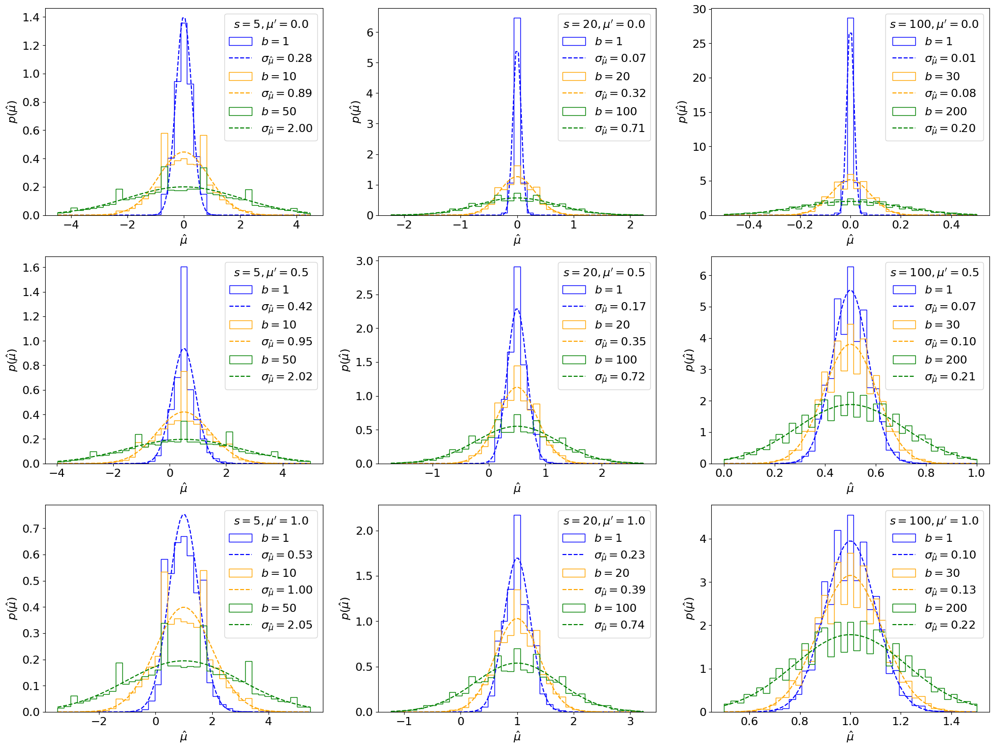
_images/ca03f3ab34ee05adc8c16ad4ff17a4761849630df53e405bb481a36e41ebf98e.png — Fig. 6.4 Asymptotic (dotted lines) and toy-based (solid lines) distributions, using 30,000 toys each, of the MLE of \(\mu\) for different \(s\), \(b\), and true signal strength \(\mu'\).#

We see that this matches well, generally, for large \(s, b\), while for small values there are more significant differences. We can also check the total per-bin errors between the asymptotic form and the toy-based distributions directly (showing here only for \(\mu' = 1\)):

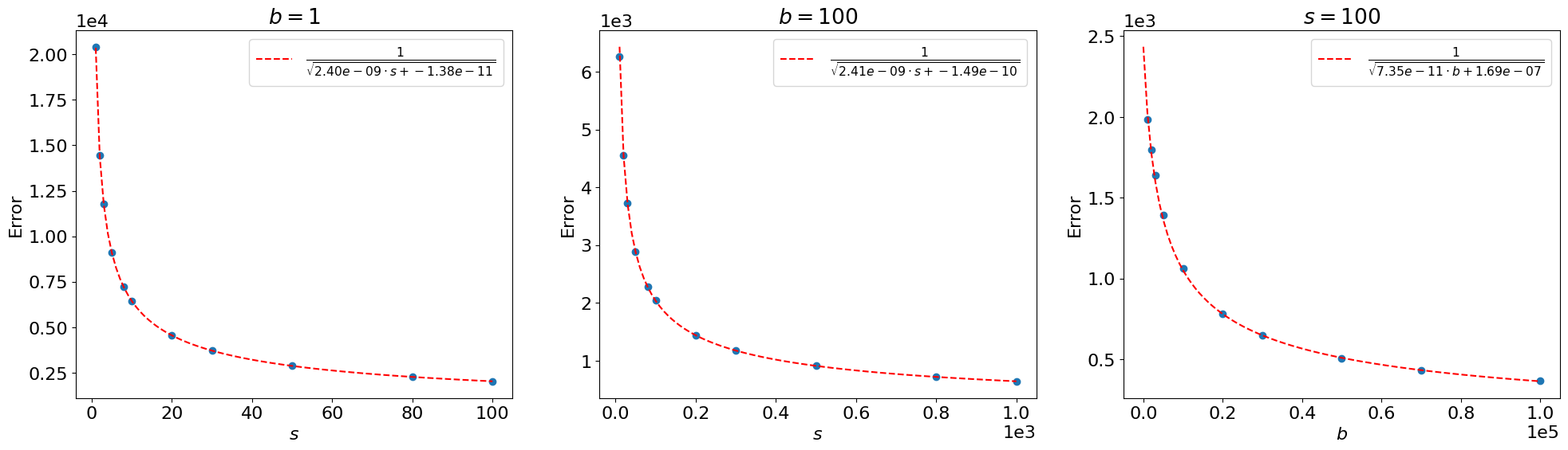
_images/a9c36843388dd1505e0013e81e09ac0990ed2d9bae3eafeff9dc64abe208876e.png — Fig. 6.5 Error between the sampled toy distributions, using 50,000 toys each, and the asymptotic distributions of the MLE of \(\mu\) for different \(s\) and \(b\) (blue), for the nominal signal strength \(\mu' = 1\). and \(1/\sqrt{N}\) fits (red).#

The error scales as \(\sim \frac{1}{\sqrt{s}}\) and \(\sim \frac{1}{\sqrt{b}}\), as we claimed above.

6.6. Numerical estimation and the Asimov dataset#

For our simple model, we were able to derive the Fisher information \(\mathcal I\) and, hence, the asymptotic form of \(\hat \mu\) analytically. In general, however, this is not possible and instead we have to minimize \(l\), find its second derivatives, and solve Eq. (6.4) etc. numerically. But how do we deal with the expectation value over the observed data (\(n, m\) in our case)? Naively, this would require averaging over a bunch of generated toy \(n, m\) values again, which defeats the purpose of using the asymptotic form of \(\hat \mu\)!

Instead, we can switch the order of operations in Eq. (6.4) and rewrite it as:

(6.9)#\[ \mathcal I_{ij}(\mu, b) = - \mathbb E[\partial^i\partial^j l(\mu, b; n, m)] = - \partial^i\partial^j \mathbb E[l(\mu, b; n, m)] = -\partial^i\partial^j l(\mu, b; \mathbb E[n], \mathbb E[m]). \]

Importantly, this says we can find \(\mathcal I\) by simply evaluating the likelihood for a dataset of observations equal to their expectation values under \(\mu'\) instead of averaging over the distribution of observations and then getting its second derivatives.

Definition

Such a dataset is called the Asimov dataset, and \(L(\mu; \mathbb E[n], \mathbb E[m]) \equiv L_A\) is referred to as the “Asimov likelihood”.

6.7. Summary#

We derived the asymptotic form of the probability distribution of the MLE \(\hat\mu\) of the POI \(\mu\), \(p(\hat\mu)\), which is a Gaussian centered at the true value \(\mu'\) with a variance equal to the inverse of the Fisher information matrix: \(\hat\mu - \mu' \simeq N(0, \sqrt{\mathcal I^{-1}_{\mu\mu}(\mu', b')})\). We also discussed the important concept of the Asimov dataset, where all observations are equal to their expectation values under \(\mu'\), for simplifying the numerical evaluation of \(\mathcal I^{-1}_{\mu\mu}(\mu', b')\). Next, we use the above to derive the asymptotic form of the profile likelihood ratio in Chapter 7.