Asymptotic Form of the Profile Likelihood Ratio

7. Asymptotic Form of the Profile Likelihood Ratio#

7.1. Recap#

7.1.1. Data model#

We have been working with a probability model and likelihood function for a simple one bin counting experiment with $n$ observed, $s$ expected signal, and $b$ expected background events in our signal region and $m$ observed and $b$ expected background events, in our control region, with the signal strength parametrized by $\mu$:

(7.1)#\[ P(n, m; \mu s, b) = \mathrm{Pois}(n; \mu s + b)\cdot\mathrm{Pois}(m; b) = \frac{(\mu s+b)^n e^{-(\mu s+b)}}{n!} \cdot \frac{b^m e^{-b}}{m!} = L( \mu, b), \]

The negative-log-likelihood (NLL) is:

(7.2)#\[-\ln L \equiv -l = \ln n! + \ln m! + \mu s + 2b - n\ln(\mu s+b) - m \ln b.\]

The maximum likelihood estimators (MLEs) for $\mu, b$ can be found analytically here to be:

(7.3)#\[\begin{split} \hat b &= m \\ \hat \mu &= \frac{n - m}{s} \end{split}\]

7.1.2. Test statistics#

In Part 1, we introduced the profile likelihood ratio test statistic,

(7.4)#\[ \lambda(\mu) = \frac{L(\mu, \hat{\hat{b}}(\mu))}{L(\hat{\mu}, \hat{b})}, \quad t_\mu=-2\ln \lambda(\mu), \]

(and its similar variations) and showed how quantify the compatibility of an observation based on the $p$-value $p_\mu$ of the observed test statistic $t_\mathrm{obs}$ with a particular signal hypothesis $H_\mu$:

(7.5)#\[ p_\mu = \int_{t_\mathrm{obs}}^{\infty}p(\tilde{t}_\mu|\mu)\mathrm d \tilde{t}_\mu = 1 - F(t_\mathrm{obs}|\mu) \]

and it’s associated significance.

7.1.3. Asymptotic form of the MLE#

As the toy-based approach of estimating these sampling distributions can be computationally intractable for complex models, in the previous part, we discussed the use of asymptotic - in the large-sample limit - approximations of these distributions instead. We have began this by deriving the asymptotic form of the MLE $\hat\mu$ of $\mu$:

(7.6)#\[ \hat\mu \simeq \mathcal N(\mu', \sqrt{\mathcal I^{-1}_{\mu\mu}(\mu', b')}), \]

where $\mu'$ is the true signal strength, and $\mathcal I(\mu', b')$ is the Fisher information, or covariance, matrix

(7.7)#\[ \mathcal I_{ij}(\mu', b') = - \mathbb E [\frac{\partial^2 l(\mu', b')}{\partial \mu_i \partial \mu_j}] \]

The asymptotic form is correct up to terms of order $\mathcal O(\frac{1}{\sqrt{N}})$, where $N$ represents the data sample size.

Code from previous parts:

Show code cell source Hide code cell source

def get_toys_sb(s, b, num_toys):
    """Generate toy data for a given s and b"""
    # sample n, m according to our data model (Eq. 1)
    n, m = poisson.rvs(s + b, size=num_toys), poisson.rvs(b, size=num_toys)
    return n, m


def get_toys(s, n_obs, m_obs, num_toys):
    """Generate toy data for a given s and observed n and m"""
    #  use b^^ for p(t_s|s) as recommended by Ref. 2
    b = bhathat(s, n_obs, m_obs)
    return get_toys_sb(s, b, num_toys)


def get_p_ts(test_s, n_obs, m_obs, num_toys, toy_s=None):
    """
    Get the t_tilde_s test statistic distribution via toys.
    By default, the s we're testing is the same as the s we're using for toys,
    but this can be changed if necessary (as you will see later).
    """
    if toy_s is None:
        toy_s = test_s
    n, m = get_toys(toy_s, n_obs, m_obs, num_toys)
    return t_tilde_s(test_s, n, m)


def get_ps_val(test_s, n_obs, m_obs, num_toys, toy_s=None):
    """p value"""
    t_tilde_ss = get_p_ts(test_s, n_obs, m_obs, num_toys, toy_s)
    t_obs = t_tilde_s(test_s, n_obs, m_obs)
    p_val = np.mean(t_tilde_ss > t_obs)
    return p_val, t_tilde_ss, t_obs


def get_Z(pval):
    """Significance"""
    return norm.ppf(1 - pval)


def get_p_qs(test_s, n_obs, m_obs, num_toys, toy_s=None):
    """
    Get the q_tilde_s test statistic distribution via toys.
    By default, the s we're testing is the same as the s we're using for toys,
    but this can be changed if necessary (as you will see later).
    """
    if toy_s is None:
        toy_s = test_s
    n, m = get_toys(toy_s, n_obs, m_obs, num_toys)
    return q_tilde_s(test_s, n, m)


def get_pval_qs(test_s, n_obs, m_obs, num_toys, toy_s=None):
    """p value"""
    q_tilde_ss = get_p_qs(test_s, n_obs, m_obs, num_toys, toy_s)
    q_obs = q_tilde_s(test_s, n_obs, m_obs)
    p_val = np.mean(q_tilde_ss > q_obs)
    return p_val, q_tilde_ss, q_obs


def get_limits_CLs(s_scan: list, n_obs: int, m_obs: int, num_toys: int, CL: float = 0.95):
    p_cls_scan = []  # saving p-value for each s

    for s in s_scan:
        p_mu, t_tilde_sb, t_obs = get_ps_val(s, n_obs, m_obs, num_toys)
        p_b, t_tilde_sb, t_obs = get_ps_val(s, n_obs, m_obs, num_toys, toy_s=0)
        p_b = 1 - p_b
        p_cls_scan.append(p_mu / (1 - p_b))

    # find the values of s that give p_value ~= 1 - CL
    pv_cl_diff = np.abs(np.array(p_cls_scan) - (1 - CL))
    half_num_s = int(len(s_scan) / 2)
    s_low = s_scan[np.argsort(pv_cl_diff[:half_num_s])[0]]
    s_high = s_scan[half_num_s:][np.argsort(pv_cl_diff[half_num_s:])[0]]

    return s_low, s_high


def get_upper_limit_CLs(s_scan: list, n_obs: int, m_obs: int, num_toys: int, CL: float = 0.95):
    p_cls_scan = []  # saving p-value for each s

    for s in s_scan:
        p_mu, q_tilde_sb, q_obs = get_pval_qs(s, n_obs, m_obs, num_toys)
        p_b, q_tilde_sb, q_obs = get_pval_qs(s, n_obs, m_obs, num_toys, toy_s=0)
        p_b = 1 - p_b
        p_cls_scan.append(p_mu / (1 - p_b))

    # find the values of s that give p_value ~= 1 - CL
    pv_cl_diff = np.abs(np.array(p_cls_scan) - (1 - CL))
    s_upper = s_scan[np.argsort(pv_cl_diff)[0]]

    return s_upper


def get_asym_std(mu, s, b):
    """Inputs should be the "true" mu and b values"""
    return np.sqrt(mu * s + 2 * b) / s

7.2. Introduction#

We now build on Chapter 6 to derive the asymptotic form of the sampling distribution $p(t_\mu|\mu')$ of the profile likelihood ratio test statistic $t_\mu$, under a “true” signal strength of $\mu'$. This asymptotic form is extremely useful for simplifying the computation of (expected) significances, limits, and intervals; indeed, standard procedure at the LHC is to use it in lieu of toy-based, empirical distributions for $p(t_\mu|\mu')$.

We’ll first derive the asymptotic form of $t_\mu$, which we’ll find depends on the variance $\sigma_{\hat\mu}^2$ of the MLE $\hat\mu$. We’ll then discuss the formula for $p(t_\mu|\mu')$, and cover two methods for estimating $\sigma_{\hat\mu}^2$ that both make use of the Asimov dataset from Chapter 6.6. We’ll finally apply the asymptotic CDF of $p(t_\mu|\mu')$ to the simple examples of hypothesis testing from Chapter 3.

7.3. Asymptotic form of the profile likelihood ratio#

We now derive the asymptotic form of the profile likelihood ratio test statistic $t_\mu$ (Eq. (7.4)) by following a similar procedure to Chapter 6 - and using the previous results - of Taylor expanding around its minimum at $\hat\mu$:

(7.8)#\[\begin{split} t_\mu &= -2\ln\lambda(\mu) \\ &= -2l(\mu, \hat{\hat{b}}(\mu)) + 2l(\hat\mu, \hat{b}) \\ &\simeq \underbrace{-2l(\hat\mu, \hat{\hat{b}}(\hat\mu)) + 2l(\hat\mu, \hat{b})}_{\textcolor{blue}{\hat{\hat{b}}(\hat\mu)=\hat b \text{ so this is 0}}} - \underbrace{2l'(\hat\mu, \hat{\hat{b}}(\hat\mu))(\mu-\hat\mu)}_{\textcolor{blue}{l'(\hat\mu, \hat b) = 0}} - 2l''(\hat\mu, \hat{\hat{b}}(\hat\mu))\cdot\frac{(\mu-\hat\mu)^2}{2} \\ &= -l''(\hat\mu, \hat b) \cdot (\mu-\hat\mu)^2 \\ &= \underbrace{-\mathbb E[l''(\hat\mu, \hat b)]}_{\textcolor{blue}{\text{By law of large numbers}}} \cdot (\mu-\hat\mu)^2 \\ &= \underbrace{-\mathbb E[l''(\mu', b')]}_{\textcolor{blue}{\text{Since bias of MLEs $\sim$ 0}}} \cdot (\mu-\hat\mu)^2 \\ &= \underbrace{\mathcal I_{\mu\mu}(\mu', b')}_{\textcolor{blue}{\text{From definition of Fisher information}}} \cdot (\mu-\hat\mu)^2 \\ \Rightarrow & \underbrace{\boxed{t_\mu \simeq \frac{(\mu-\hat\mu)^2}{\sigma_{\hat\mu}^2}}}_{\textcolor{blue}{\text{Using } \sigma_{\hat\mu} \simeq \sqrt{\mathcal I^{-1}_{\mu\mu}(\mu', b')}}} + \mathcal O((\mu-\hat\mu)^3) + \mathcal O(\frac{1}{\sqrt N}). \end{split}\]

Here, just like in Eq. (6.6), we use the law of large numbers in line 5 and take $l''(\hat\mu, \hat b)$ to asymptotically equal its expectation value under the true parameter values $\mu', b'$: $l''(\hat\mu, \hat b) \xrightarrow{\sqrt{N} >> 1} \mathbb E[l''(\hat\mu, \hat b)]$. We then in line 6 also use the fact that MLEs are generally unbiased estimators of the true parameter values in the large sample limit to say $\mathbb E[l''(\hat\mu, \hat b)] \xrightarrow{\sqrt{N} >> 1} \mathbb E[l''(\mu', b')]$. Finally, in the last step we use the asymptotic form of the MLE (Eq. (7.6)).

7.4. Asymptotic form of $p(t_\mu|\mu')$#

Now that we have an expression for $t_\mu$, we can consider its sampling distribution. With a simple change of variables, the form of $p(t_\mu|\mu')$ should hopefully be evident: recognizing that $\mu$ and $\sigma_{\hat\mu}^2$ are simply constants, while $\hat\mu$ we know is distributed as a Gaussian centered around $\mu'$ with variance $\sigma_{\hat\mu}^2$, let’s define $\gamma \equiv \frac{\mu-\hat\mu}{\sigma_{\hat\mu}}$, so that

(7.9)#\[\begin{split} t_\mu &\simeq \frac{(\mu-\hat\mu)^2}{\sigma_{\hat\mu}^2} = \gamma^2, \\ \gamma &\sim \mathcal N \bigg(\frac{\mu - \mu'}{\sigma_{\hat\mu}}, 1 \bigg). \end{split}\]

For the special case of $\mu = \mu'$, we can see that $t_\mu$ is simply the square of a standard normal random variable, which is the definition of the well-known $\chi^2_k$ distribution with $k=1$ degrees of freedom (DoF):

(7.10)#\[ p(t_\mu|\mu) \sim \chi^2_1. \]

In the general case where $\mu$ may not $ = \mu'$, $t_\mu$ is the square of random variable with unit variance but non-zero mean. This is distributed as the similar, but perhaps less well-known, non-central chi-squared $\chi'^2_k(\Lambda)$, again with 1 DoF, and with a “non-centrality parameter”

(7.11)#\[ \Lambda = \bar\gamma^2 = \bigg(\frac{\mu - \mu'}{\sigma_{\hat\mu}}\bigg)^2, \]

(7.12)#\[ p(t_\mu|\mu') \sim \chi'^2_1(\Lambda). \]

The “central” vs. non-central chi-squared distributions are visualized below for $k = 1$:

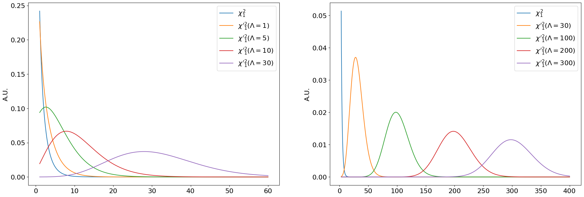
Fig. 7.1 Central $\chi^2_k$ and non-central ${\chi'}^2_k(\Lambda)$ distributions for $\Lambda$ between $1-30$ (left) and $30-300$ (right).#

We can see that $\chi'^2_k(\Lambda)$ simply shifts towards the right as $\Lambda$ increases (at $\Lambda = 0$ it is a regular central $\chi^2$). As $\Lambda \rightarrow \infty$, $\chi'^2_k(\Lambda)$ becomes more and more like a normal distribution with mean $\Lambda$.

Hopefully you can convince yourself from here - or try extending the derivation in Eq. (7.8) to multiple POIs - of the simple generalization to multiple POIs $\vec\mu$:

Result

(7.13)#\[ p(t_\mu|\mu') \sim \chi'^2_k(\Lambda), \]

where the DoF $k$ are equal the number of POIs $\dim\vec\mu$, and

(7.14)#\[ \Lambda = (\vec\mu - \vec\mu')^T \cdot \tilde{\mathcal I}^{-1}(\vec\mu') \cdot (\vec\mu - \vec\mu'), \]

where $\tilde{\mathcal I}^{-1}$ is $\mathcal I^{-1}$ restricted only to the components corresponding to the POIs.

7.5. Estimating $\sigma_{\hat\mu}^2$#

The critical remaining step to understanding the asymptotic distribution of $t_\mu$ is estimating $\sigma_{\hat\mu}^2$ to find the non-centrality parameter $\Lambda$ in Eq. (7.11). We’ll now go over two methods to this.

7.5.1. Method 1: Inverting the Fisher information / covariance matrix#

The first method is simply using $\sigma_{\hat\mu} \simeq \sqrt{\mathcal I^{-1}_{\mu\mu}(\mu', b')}$ as in Part 5. Let’s see what this looks like for our counting experiment, using the analytic form for $\sigma_{\hat\mu}$ from Eq. (6.8):

Show code cell source Hide code cell source

def plot_p_tmu(lambda_fn):
    num_toys = 30000
    s, b = 30, 10
    mus = [0, 1]  # , 1.0, 10.0]
    muprimes = [
        [0, 0.3, 0.6, 1],
        [0, 0.3, 0.6, 1],
    ]

    fig, axs = plt.subplots(1, 3, figsize=(32, 8))
    colours = ["blue", "orange", "green", "red"]

    xmaxs = [40, 80]

    for i, (mu, muprimes) in enumerate(zip(mus, muprimes)):
        axs[i].set_title(rf"Testing $\mu={mu}$ ($s = {s}, b = {b}$)")
        xmax = xmaxs[i]
        for j, muprime in enumerate(muprimes):
            # sample n, m according to our data model (Eq. 1)
            n, m = poisson.rvs(s * muprime + b, size=num_toys), poisson.rvs(b, size=num_toys)
            axs[i].hist(
                t_s(s * mu, n, m),
                np.linspace(0, xmax, 41),
                histtype="step",
                density=True,
                label=rf"$\mu'={muprime}$",
                color=colours[j],
            )

            x = np.linspace(xmax / 160, xmax, 101)

            if mu == muprime:
                axs[i].plot(
                    x, chi2.pdf(x, 1), label=r"$\chi^2_1$", color=colours[j], linestyle="--"
                )
            else:
                l = lambda_fn(mu, muprime, s, b)
                axs[i].plot(
                    x,
                    ncx2.pdf(x, 1, l),
                    label=rf"$\chi'^2_1(\Lambda = {l:.1f})$",
                    color=colours[j],
                    linestyle="--",
                )

        axs[i].legend()
        axs[i].set_xlabel(r"$t_\mu$")
        axs[i].set_ylabel(r"$p(t_\mu|\mu')$")

    i = 2
    sbmumups = [(300, 100, 1, 0), (20, 10, 3, 0), (10, 10, 1, 30)]
    xmax = 600

    for j, (s, b, mu, muprime) in enumerate(sbmumups):
        # sample n, m according to our data model (Eq. 1)
        n, m = poisson.rvs(s * muprime + b, size=num_toys), poisson.rvs(b, size=num_toys)
        axs[i].hist(
            t_s(s * mu, n, m),
            np.linspace(0, xmax, 41),
            histtype="step",
            density=True,
            label=rf"$s = {s}, b = {b}, \mu = {mu}, \mu'={muprime}$",
            color=colours[j],
        )

        x = np.linspace(xmax / 160, xmax, 101)

        if mu == muprime:
            axs[i].plot(x, chi2.pdf(x, 1), label=r"$\chi^2_1$", color=colours[j], linestyle="--")
        else:
            l = lambda_fn(mu, muprime, s, b)
            axs[i].plot(
                x,
                ncx2.pdf(x, 1, l),
                label=rf"$\chi'^2_1(\Lambda = {l:.1f})$",
                color=colours[j],
                linestyle="--",
            )

    axs[i].set_ylim(0, 0.03)
    axs[i].legend()
    axs[i].set_xlabel(r"$t_\mu$")
    axs[i].set_ylabel(r"$p(t_\mu|\mu')$")

    plt.show()

def LambdaFisher(mu, muprime, s, b):
    """
    Non-centrality parameter of the asymptotic non-central chi-squared distribution of p(t_mu),
    estimated using the inverse of the Fisher information matrix.
    """
    return np.power((mu - muprime) / get_asym_std(muprime, s, b), 2)


plot_p_tmu(LambdaFisher)

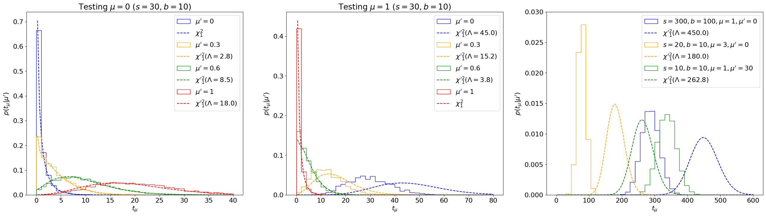
Fig. 7.2 Comparing the distribution $p(t_\mu|\mu')$ (solid) with non-central ${\chi'}_1^2(\Lambda)$ distributions (dotted) for a range of $s, b, \mu, \mu'$ values, with $\sigma^2_\hat\mu$ estimated using the inverse of the Fisher information matrix.#

We can see that this asymptotic approximation agrees well with the true distribution for some range of parameters, but can deviate significantly for others, as highlighted especially in the right plot.

7.5.2. Interlude on Asimov dataset#

While we are able to find the analytic form for $\sqrt{\mathcal I^{-1}_{\mu\mu}(\mu', b')}$ easily for our simple counting experiment, in general it has to be calculated numerically. As introduced in Chapter 6.6, to deal with the expectation value under $\mu', b'$ in Eq. (7.7), we can make use of the Asimov dataset, where the observations $n_A$, $m_A$ are taken to be their expectation values under $\mu', b'$, simplifying the calculation of $\mathcal I$ to Eq. (6.9).

Explicitly, for our counting experiment (Eq. (7.1)), the Asimov observations are simply

(7.15)#\[\begin{split} n_A &= \mathbb E[n] = \mu' s + b' \\ m_A &= \mathbb E[m] = b'. \end{split}\]

We’ll now consider a second powerful use of the Asimov dataset to estimate $\sigma^2_{\hat\mu}$.

7.5.3. Method 2: The “Asimov sigma” estimate#

Putting together Eqs. (7.3) and (7.15), we can derive a nice property of the Asimov dataset: the MLEs $\hat\mu$, $\hat b$ equal the true values $\mu'$, $b'$:

(7.16)#\[\begin{split} \hat b &= m_A = b' \\ \hat \mu &= \frac{n_A - m_A}{s} = \frac{\mu's + b' - b'}{s} = \mu'. \end{split}\]

Thus, $t_\mu$ evaluated for the Asimov dataset is exactly the non-centrality parameter $\Lambda$ that we are after!

(7.17)#\[ t_{\mu, A} \simeq \bigg (\frac{\mu-\hat\mu}{\sigma_{\hat\mu}}\bigg)^2 = \bigg (\frac{\mu-\mu'}{\sigma_{\hat\mu}}\bigg)^2 = \Lambda. \]

While, not strictly necessary to obtain the asymptotic form for $p(t_\mu|\mu')$, we can also invert this to estimate $\sigma_{\hat\mu}$, as

(7.18)#\[ \sigma_A \simeq \frac{(\mu-\mu')^2}{t_{\mu, A}}, \]

where $\sigma_A$ is called the “Asimov sigma”.

We plot below the asymptotic distributions using $\Lambda \simeq t_{\mu, A}$:

def LambdaA(mu, muprime, s, bprime):
    """
    Non-centrality parameter of the asymptotic non-central chi-squared distribution of p(t_mu),
    estimated using the test statistic for the Asimov dataset n = E[n] = µ's + b', m = E[m] = b'
    """
    return t_s(s * mu, s * muprime + bprime, bprime)


plot_p_tmu(LambdaA)

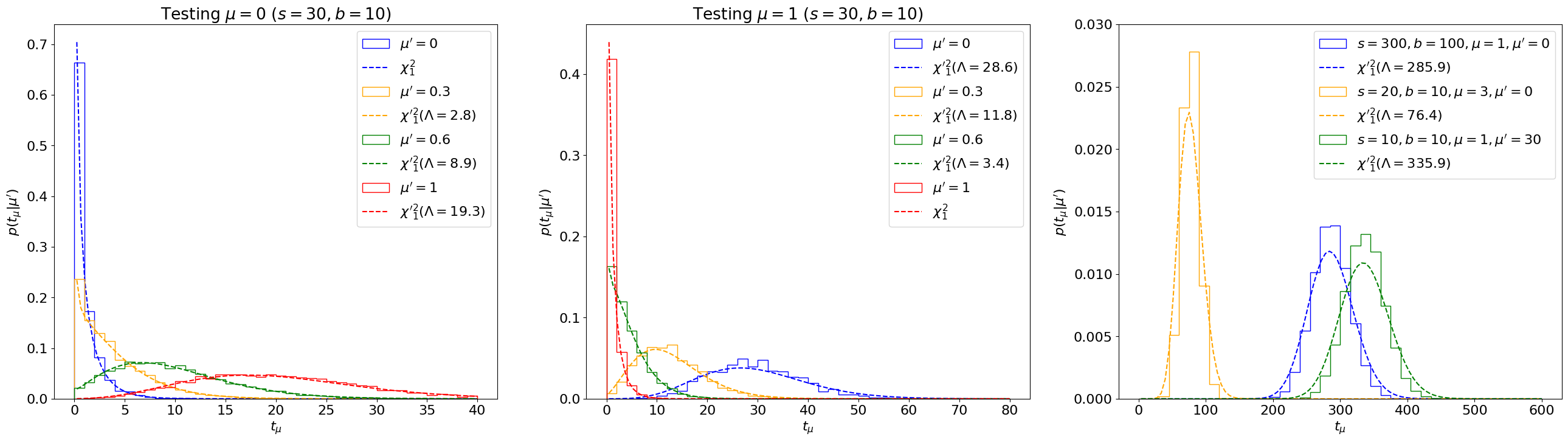
Fig. 7.3 Comparing the sampling distribution $p(t_\mu|\mu')$ with non-central ${\chi'}_1^2(\Lambda)$ distributions for a range of $s, b, \mu, \mu'$ values, with the Asimov sigma estimation for $\sigma^2_\hat\mu$.#

We see that this estimate matches the sampling distributions very well, even for cases where the covariance-matrix-estimate failed! Indeed, this is why estimating $\sigma_{\hat\mu} \simeq \sigma_A$ is the standard in LHC analyses, and that is the method we’ll employ going forward.

Important

Despite the pervasive use of the asymptotic formula at the LHC, it’s important to remember that it’s an approximation, only valid for large statistics. We can see how it breaks down for $s, b \lesssim 10$ below.

plot_p_tmu_sb(LambdaA)

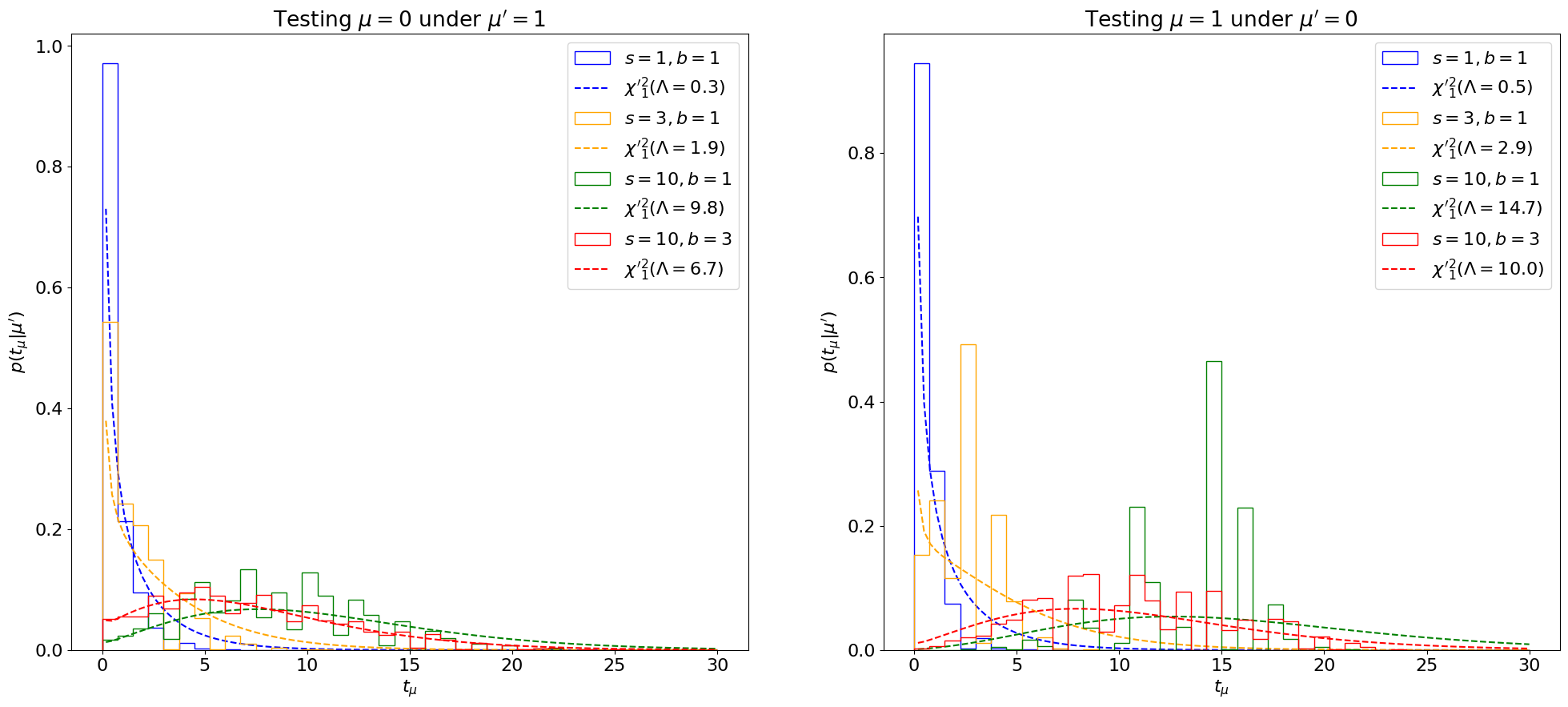
Fig. 7.4 Comparing the sampling distribution $p(t_\mu|\mu')$ with non-central ${\chi'}_1^2(\Lambda)$ distributions for different $s, b \leq 10$, showing the break-down of the $\sigma_A$ approximation for $\sigma^2_\hat\mu$ at low statistics.#

7.6. The PDF and CDF#

The probability distribution function (PDF) for a $\chi'^2_k(\Lambda)$ distribution can be found on e.g. Wikipedia as being (for $k=1$ here):

(7.19)#\[ p(t_\mu|\mu') \simeq \chi'^2_1(\Lambda) = \frac{1}{2\sqrt{t_\mu}}\big(\varphi(\sqrt{t_\mu} - \sqrt\Lambda) + \varphi(\sqrt{t_\mu} + \sqrt\Lambda)\big), \]

where $\varphi$ is the PDF of a standard normal distribution.

For $\mu = \mu' \Rightarrow \Lambda = 0$, this simplifies to:

(7.20)#\[ p(t_\mu|\mu) \simeq \chi^2 = \frac{1}{\sqrt{t_\mu}}\varphi(\sqrt{t_\mu}). \]

The cumulative distribution function (CDF), again from Wikipedia (and $k=1$) is:

(7.21)#\[ F(t_\mu|\mu') \simeq \Phi(\sqrt{t_\mu} - \sqrt\Lambda) + \Phi(\sqrt{t_\mu} + \sqrt\Lambda) - 1, \]

where $\Phi$ is the CDF of the standard normal distribution.

For $\mu = \mu' \Rightarrow \Lambda = 0$, again this simplifies to:

(7.22)#\[ F(t_\mu|\mu) \simeq 2\Phi(\sqrt{t_\mu}) - 1. \]

From Eq. (7.5), we know the $p$-value $p_\mu$ of the observed $t_\mu^\mathrm{obs}$ under a signal hypothesis of $H_\mu$ is

(7.23)#\[ p_\mu = 1 - F(t_\mu^\mathrm{obs}|\mu) = 2(1 - \Phi(\sqrt{t_\mu^\mathrm{obs}})), \]

with an associated significance

(7.24)#\[ Z = \Phi^{-1}(1-p_\mu) = \Phi^{-1}(2\Phi(\sqrt{t_\mu^\mathrm{obs}} - 1) \]

7.7. Application to hypothesis testing#

Let’s see how well this approximation with toy-based $p$-values we were finding in Chapter 3.4. For the same counting experiment example, where we expect $s = 10$ and observe $n_\mathrm{obs} = 20$, $m_\mathrm{obs} = 5$, we found the $p$-value for testing the $\mu = 1$ hypothesis $p_{\mu = 1} = 0.3$ (and the associated significance $Z = 0.52$).

Using the asymptotic approximation:

def p_mu_asym(mu, s, n, m):
    """The p-value of the observations n and m under the mu signal strength hypothesis using the asymptotic approximation"""
    t_obs = t_s(mu * s, n, m)
    return 2 * (1 - norm.cdf(np.sqrt(t_obs)))


p_value_res = p_mu_asym(1, 10, 20, 5)
Z = norm.ppf(1 - p_value_res)
display(Latex(f"$p_\mu = {p_value_res:.2f}, Z = {Z:.2f}$"))

\[p_\mu = 0.30, Z = 0.52\]

We see that it agrees exactly! We can check more generally, varying $s, \mu, n_\mathrm{obs}, m_\mathrm{obs}$:

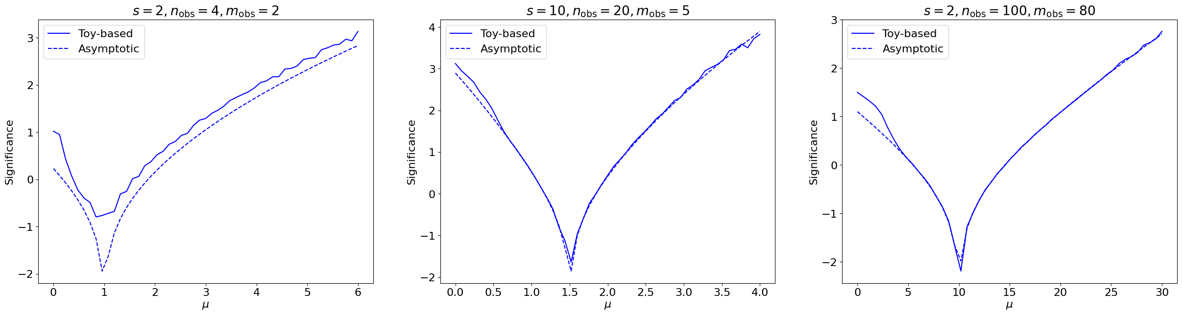
Fig. 7.5 Comparing the significances, as a function of the signal strength $\mu$ of the hypothesis being tested, for simple counting experiments with different $s, n_\mathrm{obs}, m_\mathrm{obs}$’s, derived using 30,000 toys each (solid) to estimate the $p(t_\mu|\mu)$ distribution vs. the asymptotic approximation (dashed).#

We observe generally strong agreement, except for low $n, m$ where, as expected, the asymptotic approximation breaks down.

7.8. Summary#

We have been able to find the asymptotic form for the profile-likelihood-ratio test statistic $t_\mu \simeq \frac{(\mu-\hat\mu)^2}{\sigma_{\hat\mu}^2}$, which is distributed as a non-central chi-squared ($\chi'^2_k(\Lambda)$) distribution. We discussed two methods for finding the non-centrality parameter $\Lambda$, out of which the Asimov sigma $\sigma_A$ estimation generally performed better. Finally the asymptotic formulae were applied to simple examples of hypothesis testing to check the agreement with toy-based significances. In the next part, we will discuss asymptotic formulae for the alternative test statistics for positive signals $\tilde{t}_\mu$ and upper-limit-setting $\tilde{q}_\mu$.