

7.1 Introduction
Machine learning (ML) and deep learning (DL) are revolutionizing data analysis, computing, and even real-time triggers in high-energy physics (HEP). Significant contributions of this dissertation include ML advancements for Higgs boson searches and beyond and fast detector simulations for the HL-LHC. In this chapter, to motivate them, we introduce some core concepts of ML, especially as they relate to HEP applications.
ML refers to a general class of algorithms that “learn” from data to solve problems. This is in contrast to traditional, hand-engineered bespoke algorithms designed by domain experts to address specific tasks. A relevant example in HEP is selecting a high-purity, in terms of signal versus background, region of data: a traditional approach would be to manually define a set of selections on individual kinematic features based on physical reasoning; for example, when measuring Higgs boson production, we select for events exhibiting resonances around the Higgs mass.
However, as we enter the regime of extremely large quantities of high-dimensional data and measurements of ever more complex processes (such as the searches described in this dissertation), it soon becomes intractable, or at least suboptimal, to manually define selections over the (10–100) event features that can help distinguish signal from background. This is where we turn to ML algorithms, such as boosted decision trees (BDTs) [209], which can automatically compute optimal, non-linear selections in this high-dimensional feature space.
More recently, the advent of artificial neural networks (ANNs) and deep learning (DL), along with increased data availability and computing power, has led to orders of magnitude increases in the dimensionality of data that can be exploited and the complexity and expressivity of the models built. A relevant example of their significant impact in HEP is in jet identification: jets are extremely high-dimensional objects, composed of hundreds of particles, tracks, and vertices each with several distinguishing features. Traditionally, this information had to be aggregated into hand-engineered, high-level features, such as the jet mass, number of prongs, and vertex displacements.
DL, on the other hand, allows us to leverage the full set of low particle- and vertex-level features. This leads to powerful classifiers that significantly outperform traditional methods and improve the sensitivity of our jet-based measurements. This is exemplified by the new jet identification algorithm we introduce in Chapter 13 and apply to searches for production in Chapter 14. As we argue in Section 7.3, DL also has the potential to alleviate the computational challenges we foresee in the HL-LHC era, particularly with respect to detector simulations, which are the focus of Part IV.
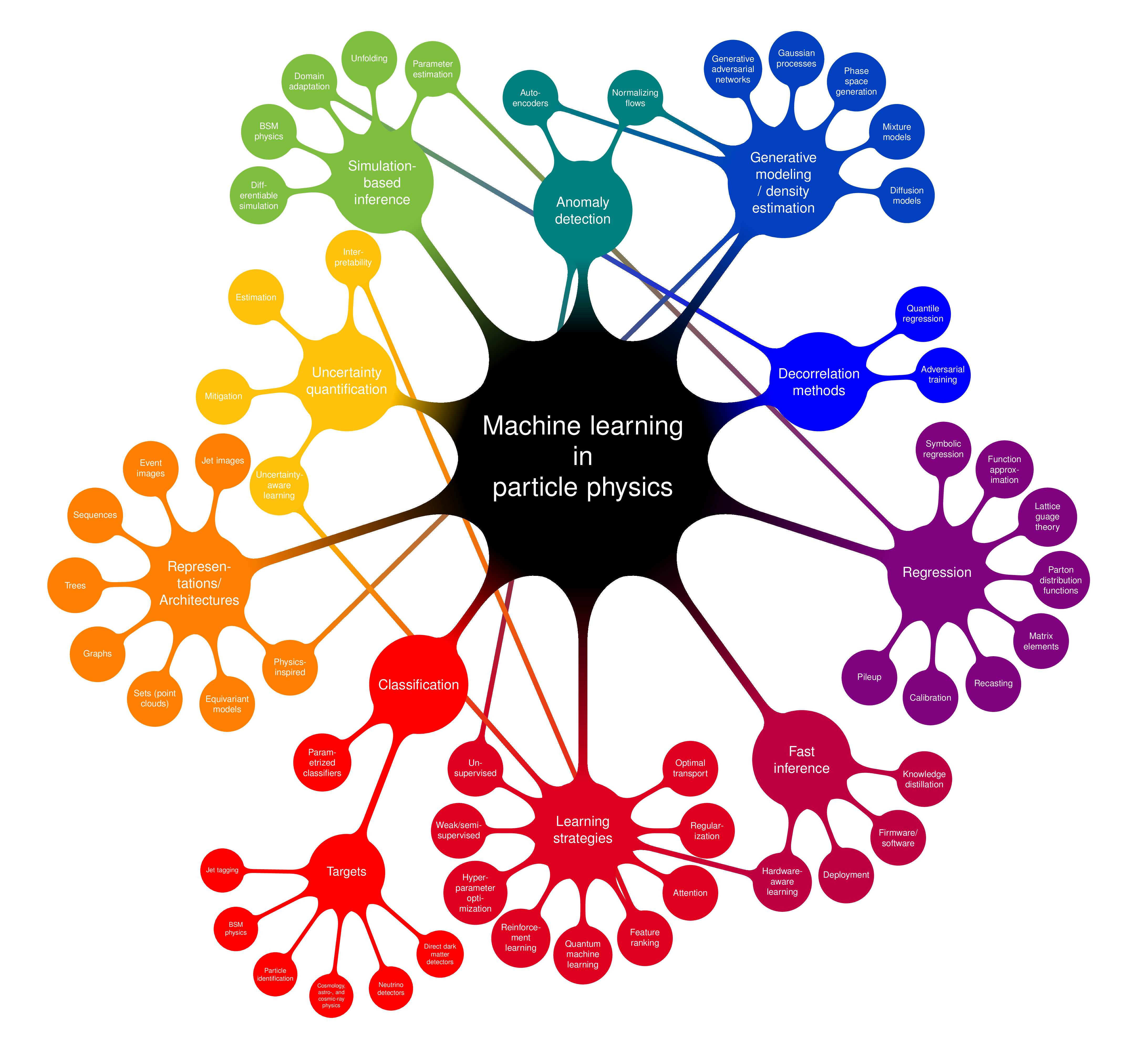
ANNs have proven to be extremely flexible building blocks out of which to construct diverse and sophisticated models for a variety of tasks in HEP, from classification and regression to simulation and anomaly detection, and more. Indeed, the development of DL algorithms in HEP is a rapidly growing subfield in its own right, and its various applications are visualized as a “nomological net” in Figure 7.1; a comprehensive “living” review is available in Ref. [210]. As we discuss below, however, with more complex data and models also comes the need for more sophisticated methods to validate, calibrate, and trust them; this is the subject of Chapters 11 and 13.3, on evaluating generative models and calibrating jet taggers, respectively.
In this chapter, we first provide a brief introduction to ML and DL, emphasizing key aspects relevant to HEP. These include the importance of: 1) generalization and calibration of models trained on simulations (Section 7.1.2); and 2) the importance of building thoughtful, physics-informed models and representations for our data (Section 7.1.4). In the same spirit, we then discuss equivariant neural networks in Section 7.2, which are designed to respect the symmetries of physical data, such as Lorentz transformations in HEP. Finally, we detail two types of unsupervised learning algorithms, autoencoders and generative models, that are relevant to the work in this dissertation in Section 7.3.
7.1.1 Basics of ML
Supervised and unsupervised learning
ML algorithms can be broadly categorized as supervised and unsupervised learning. The former involves learning a mapping between some input data and a specific output ; for example, classifying jets as originating from a Higgs boson or QCD background. Other examples include regression tasks where the target output is a continuous variable, such as predicting the mass of a jet or the energy of a particle. Algorithms used for supervised learning include support vector machines (SVMs) [211], (boosted) decision trees (BDTs) [209, 212], and neural networks. Such algorithms necessitate a labeled training dataset of input-output pairs .
Tasks for which we do not have straightforward labeled data are considered unsupervised learning problems, in which the model must learn the properties and structure of the data without explicit target outputs. Examples include clustering algorithms, which aim to group similar data points together, and generative and anomaly detection models, both of which aim to learn the underlying distribution of the data in some manner for the purposes of generating new data or identifying outliers, respectively. The latter two will be discussed in more detail in Section 7.3.
Note that these two categories are not mutually exclusive but rather two ends of a spectrum, with the middle ground including paradigms such as weakly-supervised [213] and self-supervised learning [214].
Linear models
Perhaps the simplest example of an ML task is linear regression, which entails fitting a linear model:
|
| (7.1.1) |
to a set of data points , where are the model weights which need to be learned. To do so, we define a loss function that quantifies the difference between the model’s prediction and our desired output, such as the mean squared error:
|
| (7.1.2) |
The learning objective of our model is hence to minimize with respect to the weights .
For linear regression, the minimum can in fact be found analytically to be:
|
| (7.1.3) |
where is the matrix of input data and the vector of target outputs. However, for more complex models (or even in linear regression when the matrix inversion is too expensive), numerical optimization techniques are required. The most common is gradient descent.
Gradient descent
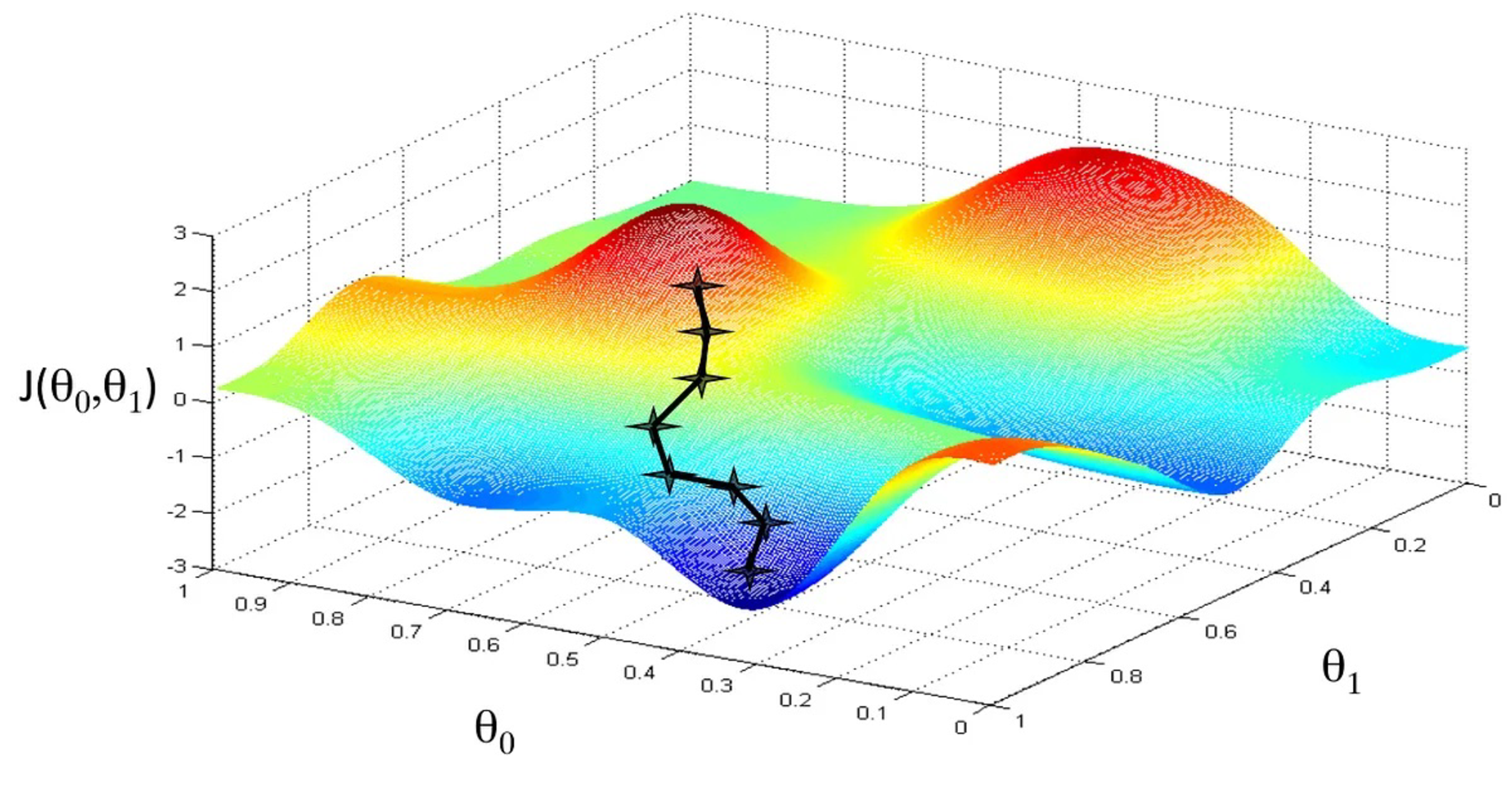
Gradient descent is an optimization algorithm that iteratively adjusts the weights of a model in the direction of steepest descent, i.e., the gradient:
|
| (7.1.4) |
where are the weights at iteration , and is the step size or learning rate (LR). This process is visualized for two learnable parameters in Figure 7.2.
Gradient descent is the backbone of all deep learning optimization algorithms; though this basic idea is typically modified to improve convergence and efficiency. The most common variants are stochastic and mini-batch gradient descent, which compute the gradient on a subset of the data at each iteration. This has the dual benefit of computational efficiency and the introduction of stochasticity into the optimization process, which can help the model escape local minima of the loss function.
Other powerful ideas include adaptive learning rates, which adjust the LR during training based on the history of the gradients and/or number of iterations; and momentum, which retains some fraction of the previous gradients to smooth out oscillations in the optimization process. Popular optimizers which incorporate these techniques include RMSprop [215] and Adam [216], both of which are prominently used for the work in this dissertation.
7.1.2 The importance of generalization and calibration
It is crucial in ML that the model not only learns the training data but can also generalize to new, unseen data. This is what signifies that the model has effectively learned the underlying patterns and relationships, rather than merely memorizing, or overfitting to, the training samples.
A standard procedure to evaluate generalization is to split the available dataset into three subsets: training, validation, and testing. The former is the only dataset used to update the learnable parameters of the model themselves, and is typically the largest subset. The validation set is used to tune hyperparameters of the model — those parameters such as model size and learning rates that cannot be “learned” through gradient descent — as well as assess the model’s performance on unseen data during training: if the performance on the validation set is significantly worse than on the training set, the model is likely overfitting. Finally, in case a bias is introduced by tuning the hyperparameters on the validation set, it is good practice to evaluate the model on the testing set at the end, which is never used to make decisions on the model.
The bias-variance tradeoff
Selecting the right model and hyperparameters involves making a bias-variance tradeoff. This is a fundamental concept in ML that describes the balance between two sources of error in a predictive model. Bias is the error due to overly simplistic assumptions in the learning algorithm — for example, using a linear model to capture non-linear relationships; while variance is the error due to a model which is too complex capturing noise in the training data.
A model with high bias may have systematic inaccuracies, or underfit the data, while a model with high variance may overfit and fail to generalize. Model selection involves using the performances on the training and validation datasets to find an optimal balance between these two errors. Common techniques to improve bias include improving the model design and increasing its complexity, while to address variance, there are several established regularization methods to reduce overfitting, such as early stopping [217], dropout [218], and batch normalization [219].
Model calibration
A related and unique aspect of ML in HEP is the reliance on theory and detector simulations to generate large quantities of labeled data for model training. The aim though, of course, is to deploy on and model correctly the real data collected by the experiments. It is hence crucial to verify how well the models generalize accurately to the latter, rather than overfitting to mismodeling in the former.
This process is sometimes referred to as calibration, where the performance of the ML model is compared between simulation and data to derive possible corrections to the model’s predictions and quantify the systematic uncertainties associated with them. As models become more complex and high-dimensional, calibration becomes increasingly challenging (and often overlooked)! To this end, significant contributions of this dissertation are the development of novel methods to efficiently and sensitively validate the performance of ML-based simulations (Chapter 11), and improving the calibration of jet identification algorithms (Chapter 13).
7.1.3 Artificial neural networks and deep learning
ANNs are ML models loosely inspired by the structure of the human brain. They were originally proposed in the 1940s, and improved over the 20th century through the perceptron [220] and backpropagation [221] algorithms, but had limited success in practical applications compared to algorithms like SVMs and decision trees.
Only in the 2010s was it recognized that their flexibility in both architecture and training makes them ideal for exploiting the recent exponential increase in data and computing power, propelling ANNs to the forefront of ML and sparking the so-called DL revolution. Through the development of large and innovative, so-called deep neural networks (DNNs), they have led to significant breakthroughs in the fields of computer vision, natural language processing, and indeed HEP. Specific types of models, or “architectures”, include convolutional neural networks (CNNs) for image data, graph neural networks (GNNs) for graph data, and transformers for sets and sequences, all of which we discuss below.
Artificial neurons and multilayer perceptrons
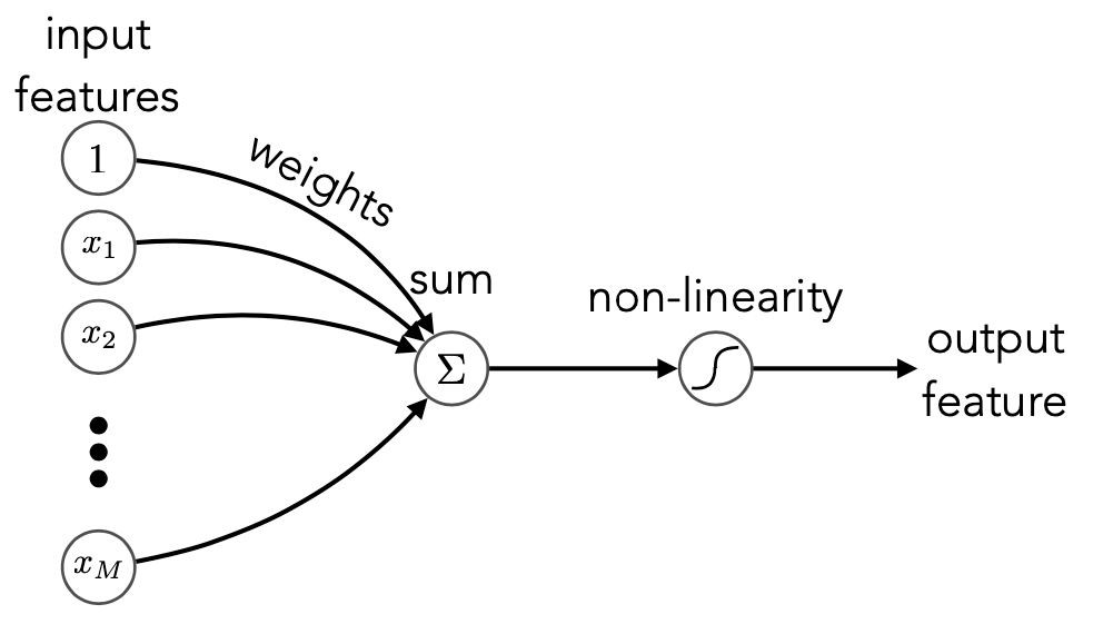
The building blocks of ANNs are single “artificial neurons”, or perceptrons [220]. They are similar to the linear models discussed above, but with an additional non-linear function — known as the activation function, applied to the output (Figure 7.3, left):
|
| (7.1.5) |
where is a constant, learned bias term. Common choices for the activation include the sigmoid, hyperbolic tangent, and piecewise linear functions.
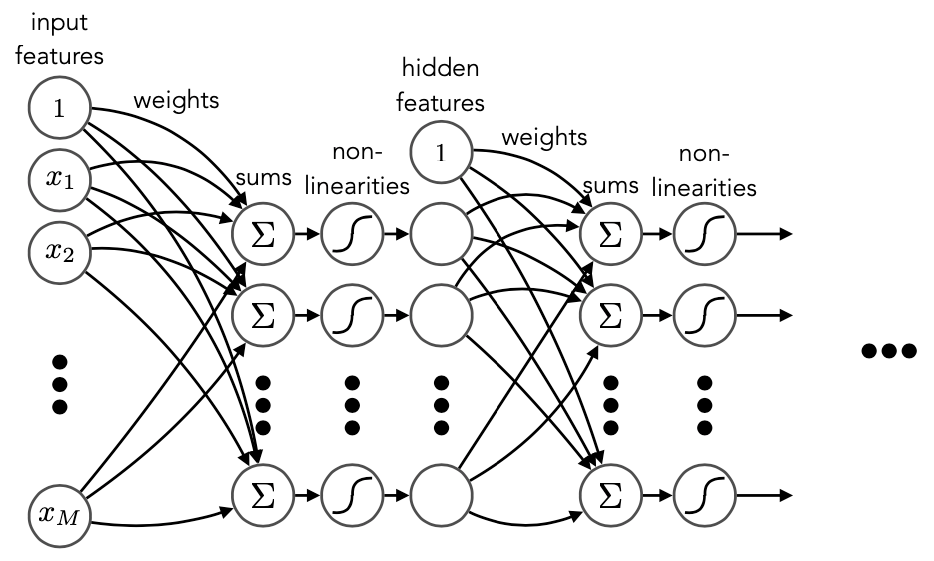
By combining multiple perceptrons in a multilayer perceptron (MLP) architecture, i.e., an ANN, we can build a powerful and flexible model capable of learning complex, non-linear relationships in the data (Figure 7.3, right). In fact, the famous universal approximation theorem [222] states that, in theory, neural networks can approximate any continuous function to arbitrary accuracy given a sufficiently large number of neurons and layers (although in practice it is not so straightforward).
Another key characteristic of ANNs is their ability to learn hierarchical representations of the data, with each layer, in principle, learning progressively more abstract features from the previous layer’s output. Intelligently designed “deep” networks with many layers can hence learn powerful, nonlinear, high-level representations of the high-dimensional input data, which can then be used to perform the desired task (assuming enough data and computing power to train them effectively). This is why this subfield of ML is also sometimes referred to as representation learning. As we discuss in Section 7.1.4, it is thus crucial to use representations and design architectures well-suited to the data and task at hand; naively adopting a specific architecture or input representation from another domain may not lead to the most optimal feature learning.
Backpropagation
Part of the effectiveness and popularity of DNNs is due to the backpropagation algorithm [221], which allows for efficient training of arbitrarily deep networks. Backpropagation is, essentially, the repeated application of the chain rule of calculus to iteratively propagate gradients of the loss function backwards through the network. For a simple two-layer network, for example:
|
| (7.1.6) |
where the superscript denotes the layer of the network, the gradient of the loss function with respect to is:
|
| (7.1.7) |
This tells us that can be computed using the gradient with respect to — which needs to be calculated anyway — and, more generally, by walking backwards through the network operations and taking the product of the derivatives at each step. This simple but powerful idea scales well to large and diverse network architectures, and is why huge DNNs can be trained effectively with relative ease.
Convolutional neural networks
We now walk through some popular ANN architectures, starting with CNNs. CNNs are a type of NN designed to process grid-like data and, particularly, images. They contributed the first major breakthrough in DL by achieving impressive performances in computer vision tasks, with models such as AlexNet [223] in 2012 and ResNet [224] in 2016.
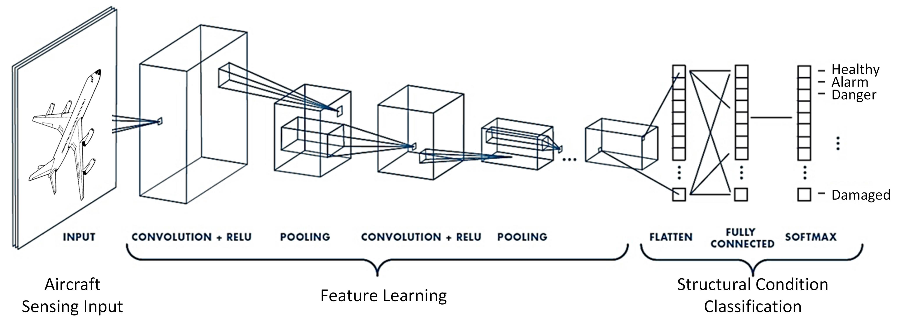
A single CNN convolutional layer convolves a set of discrete “kernels” (essentially, learnable matrices) through the input image or data (Figure 7.4), each of which detect useful features such as edges or textures. A CNN comprises multiple convolutional layers, interspersed with operations such as pooling or compression to reduce the spatial dimensions of the data, and then typically MLPs at the end as in Figure 7.4 to produce the final output.
Graph neural networks
GNNs are designed for graph-structured data, such as social networks or molecular structures. They are also useful for operating on point clouds: sets of unordered data points in some space, which we argue in Section 7.1.4 are the perfect data structures for representing particles in an event or hits in a detector. This is why GNNs have been extremely successful in HEP, generally outperforming standard MLP or CNN approaches.
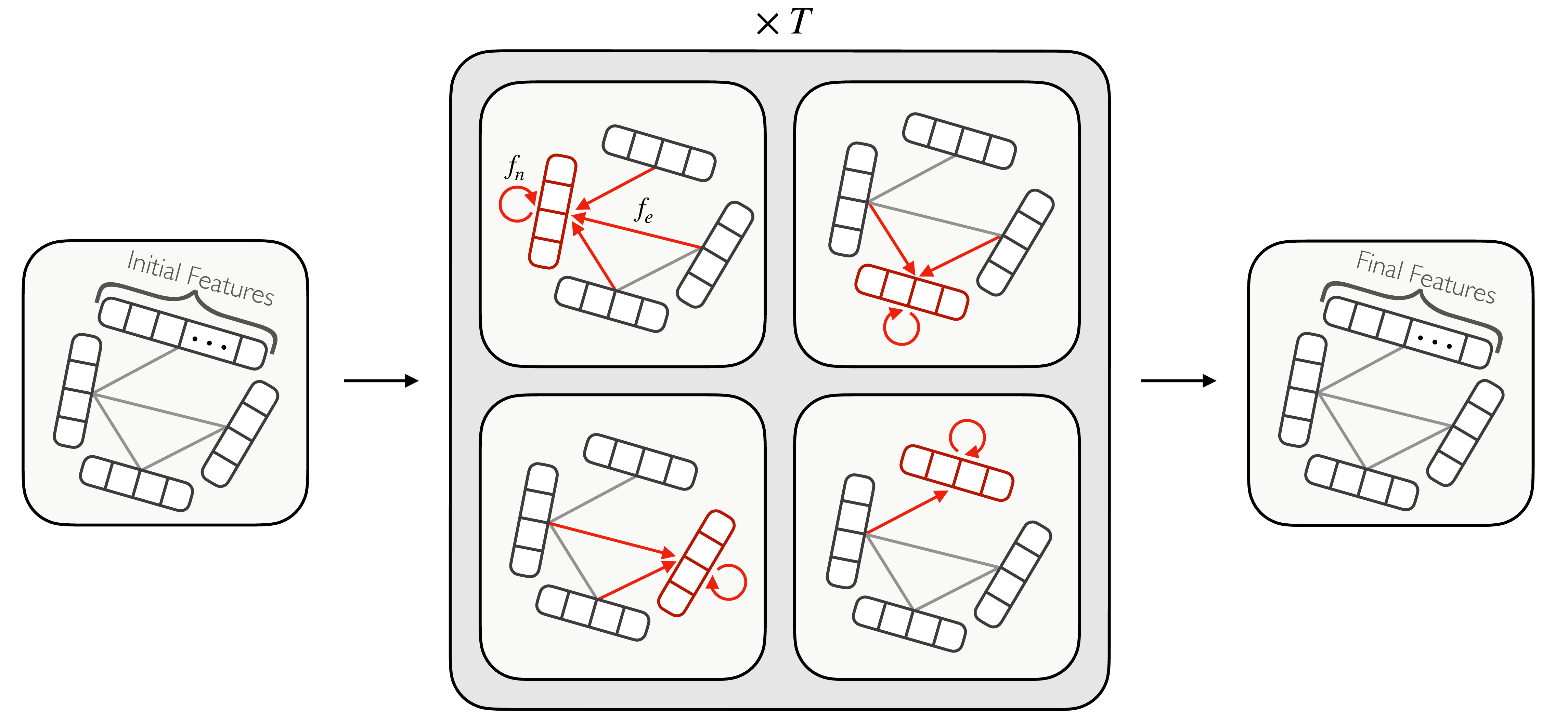
The idea behind GNNs is to learn representations per-node or per-edge, based on information aggregated from their neighbors. Some generic methods to do so include local graph convolutions — similar to CNNs, but with graph-based kernels; and message-passing neural networks (MPNNs), which deliver and aggregate learned messages between nodes. An example of an MPNN is shown in Figure 7.5, and is the basis for a novel GNN generative model introduced in Chapter 10.
Attention and transformers
The final architecture we discuss is the transformer, introduced in 2017 [225], which is the powerhouse behind the recent revolution in natural language processing (NLP) and AI chatbots such as GPT-3 [226] and its successors. Transformers are built around the idea of attention, which encourages the model to learn to attend to different parts of an input set or sequence in each layer.
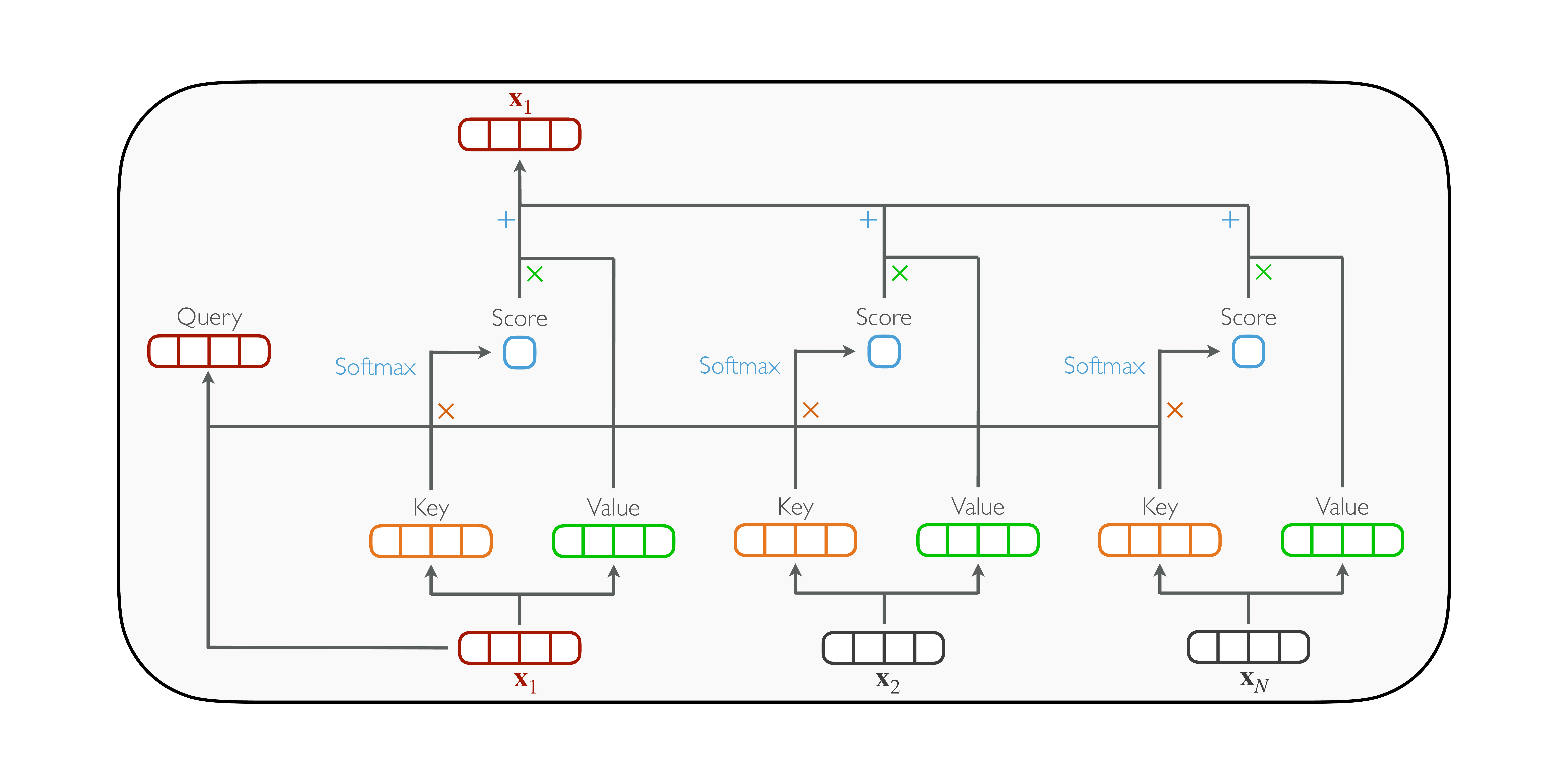
Explicitly, each element, or node’s, features in the input set are first embedded via MLPs into key () and value () pairs, while each node in the output set is embedded into a query (). The attention mechanism is then defined as:
|
| (7.1.8) |
where is the dimension of the keys and queries, and are the “attention scores” between each pair of input and output nodes. This output is finally used to update the features of the output nodes. Figure 7.6 shows a schematic of the special case of self-attention, in which the input set is also the output set; i.e., each node’s features are updated based on the features of all other nodes.
Transformers can be thought of as a type of fully-connected GNN, with attention a (particularly efficient) form of message-passing. They have proven extremely successful and durable in NLP and other sequence-based tasks, and are also gaining prominence in computer vision and HEP. We introduce two novel transformer-based models for jet simulations and tagging in Chapters 10 and 13, respectively.
7.1.4 The importance of being physics-informed
The success of specific DNN models largely depends on the in-built inductive biases — assumptions or design choices — towards certain types of data. This is why it is important in HEP to build physics-informed models and representations that respect the symmetries and biases of our data. In this section, we outline the relevant properties of HEP data, such as jets and calorimeter showers, and the inductive biases of CNNs, GNNs, and transformers, arguing that the latter two are stronger fits.
The power of CNNs, in addition to their ease of computation, comes from their biases towards natural images, namely: translation invariance — the same features are learned regardless of input translations — and locality — the convolution operation is inherently local in space, suited to the structure of natural images. This led to CNNs leading the DL revolution in the 2010s and achieving results on par with or surpassing human performance in computer vision.
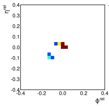
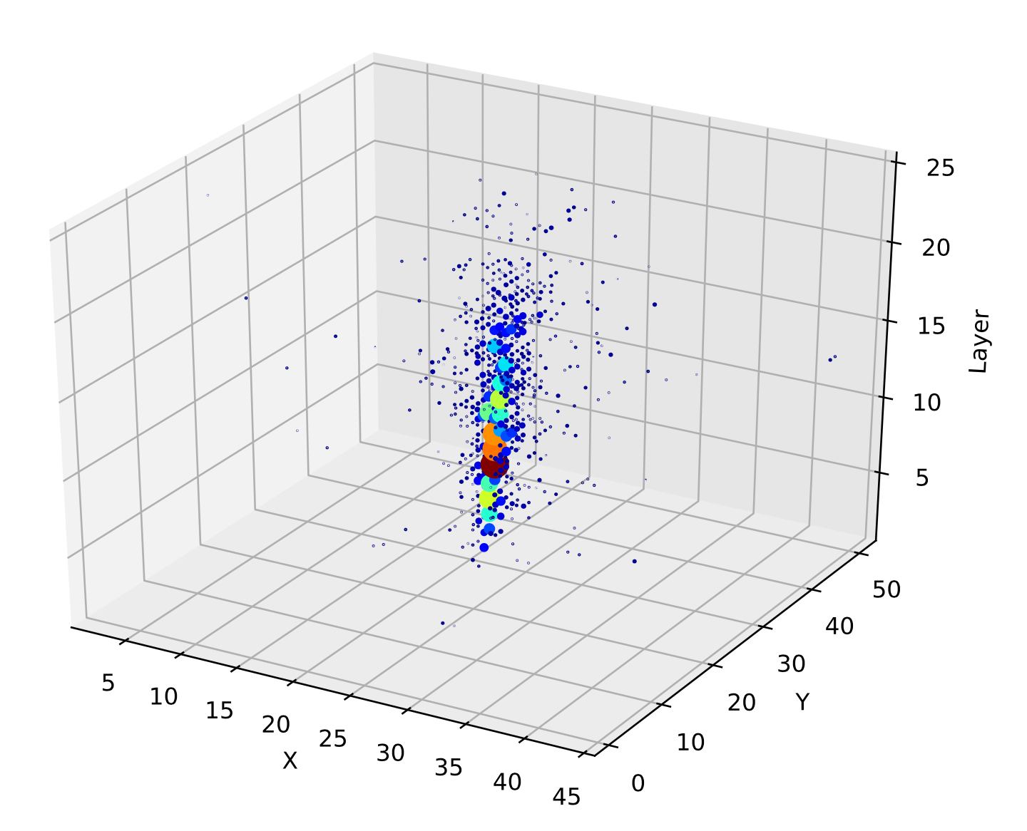
Consequently, this also led to early work in HEP applying CNNs to jets and calorimeter showers. Jets can, in principle, be represented as images by projecting the particle constituents onto a discretized angular - plane, and taking the intensity of each “pixel” in this grid to be a monotonically increasing function of the corresponding particle [227] (Figure 7.7, left). Showers can similarly be represented as 3D images of the energy deposited in the calorimeter cells (Figure 7.7, right).
At the time of the work of this dissertation, such image-based models were leading the field in tasks such as jet classification [228] and shower generation [229]. However, we argue that, despite these early successes, CNNs and images are not ideal for the physics and structure of our data, due to HEP data’s following characteristics:
- 1.
- Sparsity: particles in a jet and hits in the detector tend to be extremely sparse relative to the total angular momentum phase space and total number of cells, respectively. Indeed, we see in Figure 7.7 that the resulting “images” tend to be extremely sparse, with typically fewer than 10% of pixels nonempty [230].
- 2.
- High granularity: LHC detectors are highly granular, which means the discretization process often lowers the spatial resolution (as with the ATLAS FastCaloGAN [229]), unless the pixels are chosen to exactly match the detector cells; however, this is often computationally intractable due to the large number of cells, and the property we describe next.
- 3.
- Irregular geometry: jets and showers are not naturally square grid-like objects, and must be made to conform to this structure for use with CNNs. This is again often intractable or, at best, suboptimal.
- 4.
- Global structure: jets and particle showers each originate from a single or small set of sources, which leads to global correlations between the final-state particles and hits, independent of the spatial distance between them, that are vital to understanding the underlying physics.
Properties 1–3 strongly suggest that HEP data is not conducive to image-based representations. This is exemplified by the upcoming CMS HGCAL (Chapter 6.5.4): its high granularity, sparsity, hexagonal geometry, and non-uniform cell sizes all make HGCAL showers extremely challenging to represent as an image. Finally, Property 4 implies that local operations such as convolutions are ill-suited to the global structure of our data.
In contrast, GNNs and transformers are naturally: sparse — only the particles or hits need be represented, rather than a dense grid of mostly empty pixels; and flexible to the underlying geometry and granularity. Moreover, they are permutation invariant — learned features are independent of the order of the inputs, which means there is no need to impose an artificial ordering on particles or hits (as opposed to with an MLP, for example).
Finally, in the case of GNNs, the graph topology (i.e. the connections between nodes) can be tuned or even learned to reflect the physical nature of the data. For example, for local data, such as 3D point clouds of natural objects, connections can be defined based on the Euclidean distance between points, while in the case of jets or particle showers in a calorimeter, we can choose a fully-connected topology to reflect their global correlations (as we emphasize in Chapter 10). The attention mechanism in transformers is by definition fully connected, and hence well-suited as well.
This is why we advocate for point-cloud representations and GNN and transformer models as natural choices for HEP data. Indeed, major contributions of this dissertation are the development of the first point-cloud based generative models for jet simulations (Chapter 10), which achieve breakthrough performance for an ML simulator in terms of accuracy and efficiency, and the first transformer-based jet tagging algorithm (Chapter 13) for jet-tagging, powering a significant boost in the sensitivity of the search. Finally, in Chapter 16, we push the inductive biases of ML models further by incorporating equivariance to Lorentz-symmetries, as we introduce next.
