11.2 Experiments on gaussian-distributed data

As a first test and filtering of the many metrics discussed, we evaluate each metric’s performance on simple 2D (mixture of) Gaussian-distributed datasets. Below, we describe the specific metrics tested, the distributions we evaluate, and experimental results.

Metrics

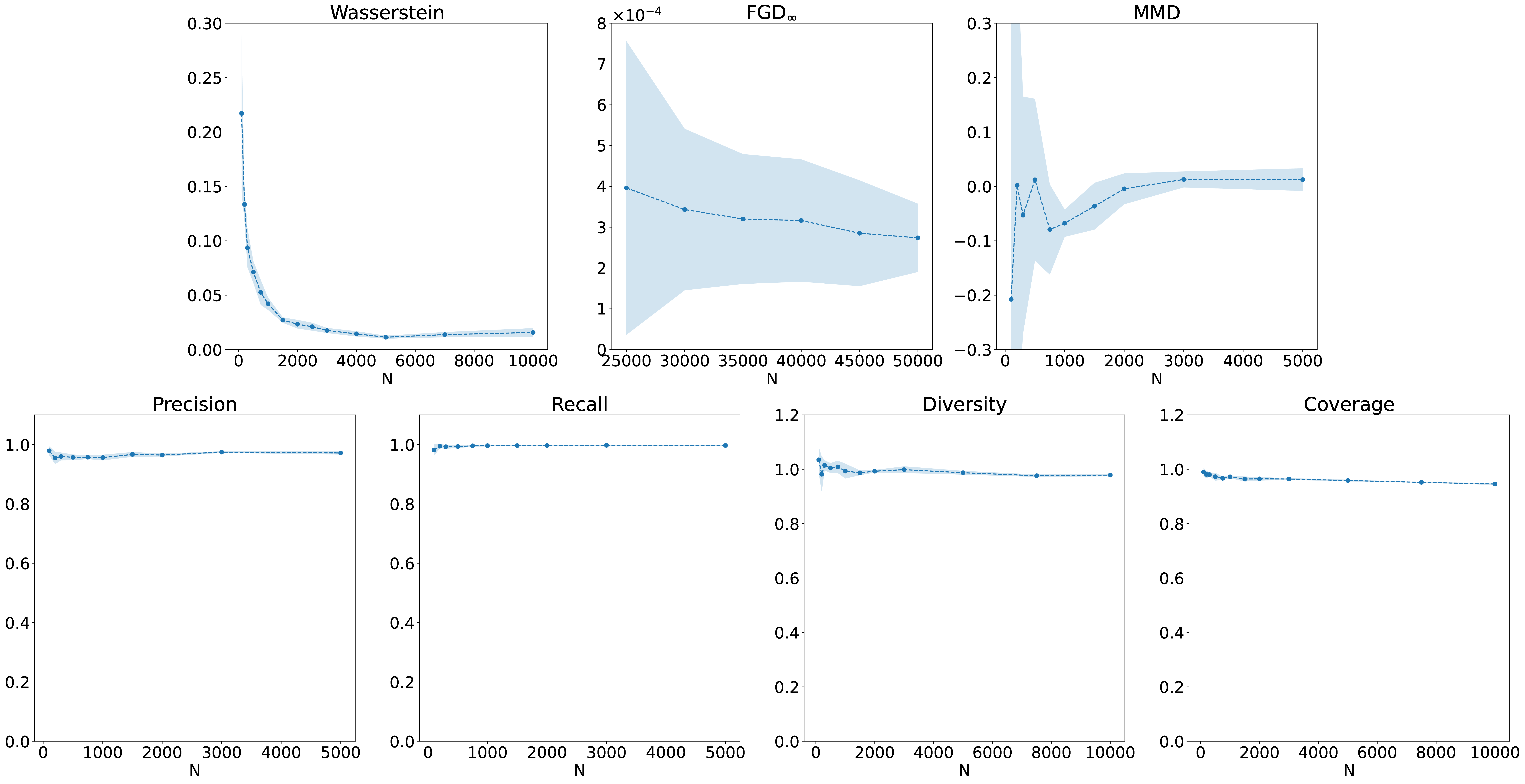
We test several metrics discussed in Section 11.1, with implementation details provided below. Values are measured for different numbers of test samples, using the mean of five measurements each and their standard deviation as the error, for all metrics but ${\mathrm{FGD}}_{\infty }$ and MMD. The sample size was increased until the metric was observed to have converged, or, as in the case of the Wasserstein distance and diversity and coverage, until it proved too computationally expensive. Timing measurements for each metric can be found in Appendix D.2.

1.

Wasserstein distance is estimated by solving the linear program described in, for example, Ref. [373], using the Python optimal transport library [374].

2.

${\mathrm{FGD}}_{\infty }$ is calculated by measuring FGD for 10 batch sizes, between a minimum batch size of 20,000 and varying maximum batch size. A linear fit is performed of the FGD as a function of the reciprocal of the batch size, and ${\mathrm{FGD}}_{\infty }$ is defined to be the $y$ intercept—it, thus, corresponds to the infinite batch size limit. The error is taken to be the standard error of the intercept. This closely follows the recommendation of Ref. [357], except empirically we find it necessary to increase the minimum batch size from 5,000 to 20,000 and to use the average of 20 measurements at each batch size in the linear fit, in order to obtain ${\mathrm{FGD}}_{\infty }$ intervals with $>$68% coverage of the true value.⁴

3.

MMD is calculated using the unbiased quadratic time estimator defined in Ref. [343]. We test 3rd (as in KID) and 4th order polynomial kernels. We find MMD measurements to be extremely sensitive to outlier sets of samples, hence we use the median of 10 measurements each per sample size as our estimates, and half the difference between the 16th and 84th percentile as the error. We find empirically that this interval has 74% coverage of the true value when testing on the true distribution.

4.

Precision and recall [361] and

5.

Diversity and coverage [362] are both calculated using the recommendations of their respective authors, apart from the maximum batch size, which we vary.

Distributions

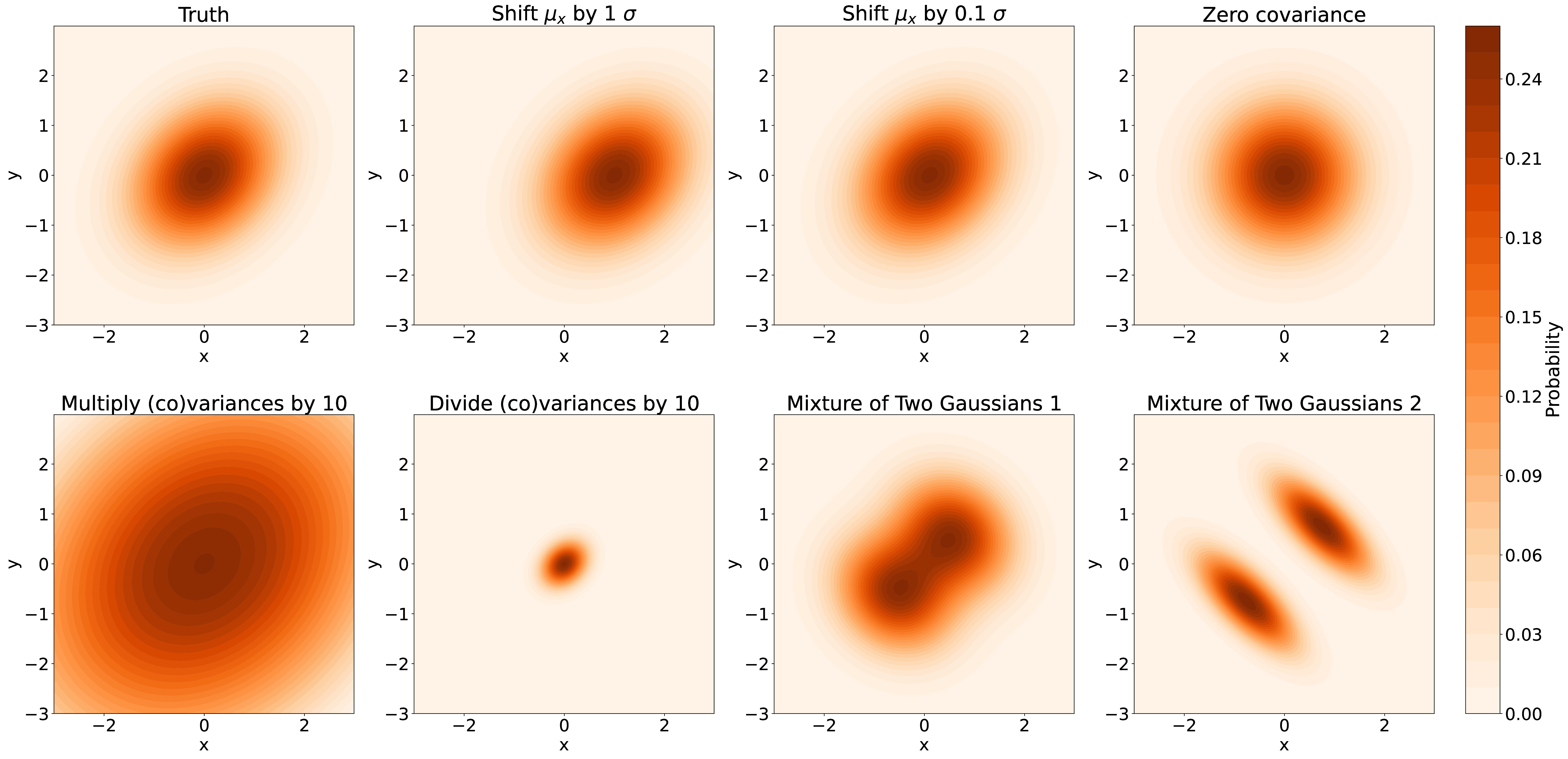
We use a 2D Gaussian with 0 means and covariance matrix $\mathrm{\Sigma }=\left(\begin{array}{cc}1.00& 0.25\\ 0.25& 1.00\end{array}\right)$as the true distribution. We test the sensitivity of the above metrics to the following distortions, shown in Figure 11.1:

1.

a large shift in $x$ (1 standard deviation $\sigma$);

2.

a small shift in $x$ ($0.1\sigma$);

3.

removing the covariance between the parameters—this tests the sensitivity of each metric to correlations;

4.

multiplying the (co)variances by 10—tests sensitivity to quality;

5.

dividing (co)variances by 10—tests sensitivity to diversity; and, finally,

6 & 7.

two mixtures of two Gaussian distributions with the same combined means, variances, and covariances as the truth—this tests sensitivity to the shape of the distribution.

Results

Bias We first discuss the performance of each metric in distinguishing between two sets of samples from the truth distribution in Figure 11.2, effectively estimating the null distributions of each test statistic. A fourth-order polynomial kernel for MMD is shown as it proved most sensitive. We see that indeed ${\mathrm{FGD}}_{\infty }$ and MMD are effectively unbiased, while the values of others depend on the sample size. This is a significant drawback; even if the same number of samples is specified for each metric to mitigate the effect of the bias, as discussed in Ref. [357], in general there is no guarantee that the level of bias for a given sample size is the same across different distributions. One possible solution is to use a sufficiently large number of samples to ensure convergence within a certain percentage of the true value. However, from a practical standpoint, the Wasserstein distance quickly becomes computationally intractable beyond $O(1000)$ samples, before which, as we see in Figure 11.2, it does not converge even for a two-dimensional distribution. Similarly, diversity and coverage require a large number of samples for convergence, which is impractical given their $O(n^2)$ scaling, while precision and recall suffer from the same scaling but converge faster.

Sensitivity Table 11.1 lists the means and errors of each metric per dataset for the largest sample size tested for each. A similar plot to Figure 11.2 for each alternative distribution can be found in Appendix D.2. A significance is also calculated for each score by assuming a Gaussian null (truth) distribution,⁵ and the most significant scores per alternative distribution are highlighted in bold. We can infer several properties of each metric from these measurements.

Focusing first on the holistic metrics (Wasserstein, ${\mathrm{FGD}}_{\infty }$, and MMD), we find that each converges to $\approx 0$ on the truth distribution, indicating their estimators are consistent. We can evaluate the sensitivity to each alternative distribution by considering the difference in scores versus the truth scores. With the notable exception of ${\mathrm{FGD}}_{\infty }$ on the mixtures of two Gaussian distributions, we observe that all three metrics find the alternatives discrepant from the truth score with a significance of $>$2 (equivalent to a $p$-value of $<$0.05 of the test statistic on the alternative distributions).

As expected, despite the clear difference in the shapes of the mixtures compared to the truth, since ${\mathrm{FGD}}_{\infty }$ has access to up to only the second-order moments of the distributions, it is not sensitive to such shape distortions. We also note that a fourth-order polynomial kernel, as opposed to the third-order kernel proposed for KID, is required for MMD to be sensitive to the mixtures of Gaussian distributions, as shown in Appendix D.2. ${\mathrm{FGD}}_{\infty }$ is, however, generally the most sensitive to other alternative distributions.

Finally, we note that precision and recall are clearly sensitive to the two distributions designed to reduce quality and diversity respectively, while not sensitive to others. This indicates that they are valuable for diagnosing these individual failure modes but not for a rigorous evaluation or comparison. Diversity and coverage are also sensitive to these distributions, but their relationship to quality and diversity is less clear. For example, the coverage is lower with the covariances multiplied by 10, when, in fact, the diversity should remain unchanged. We, therefore, conclude that precision and recall are the more meaningful metrics to disentangle quality and diversity, and use those going forward.